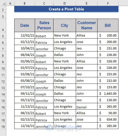
Pivot Table Custom Grouping: With 3 Criteria

We will use the following dataset to explain Custom Grouping in a Pivot Table.

What Is the Pivot Table in Excel?

A pivot table is one of the statistical tools of Microsoft Excel. It works with a large amount of data and can represent and summarize data in various ways.

In the Pivot table, we can rotate the data in the table to view from a different perspective. You don’t have to apply any further formula or other shortcuts to change the orientation of the data you want to show.

What Does Pivot Table Grouping Mean?

Grouping means organizing some data based on the same criteria such as all numerical data or text data. The Pivot table also has a grouping option. In the Pivot table, we can group data according to our needs. There is no restriction in grouping data in Excel.

How to Create a Pivot Table and Apply Grouping

Steps:

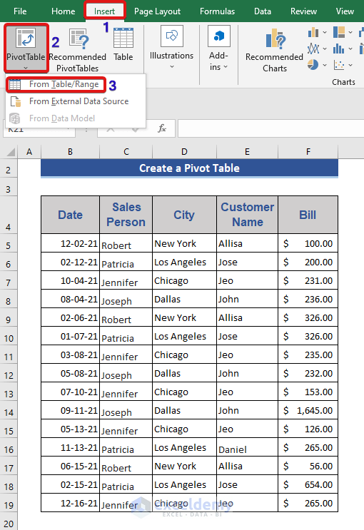
Go to the Insert tab.
Choose From Table/Range from the Pivot Table tool.

Put the range that you want to convert in the Pivot table on the Table/Range box.
Put the cell reference of the worksheet on the Location box.

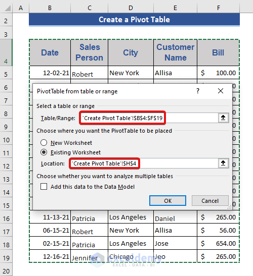
Press OK.

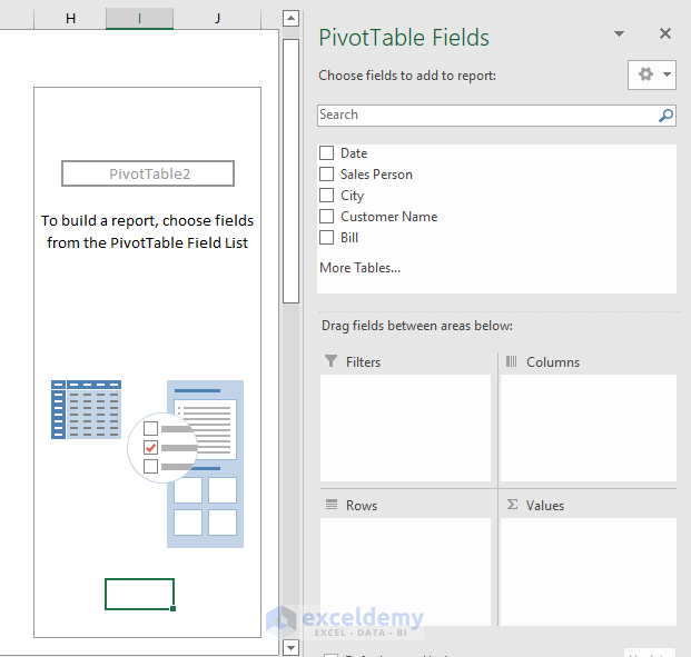
We get the PivotTable Field options. We will customize the Pivot table.

Select Sales Person and Bill from the field.

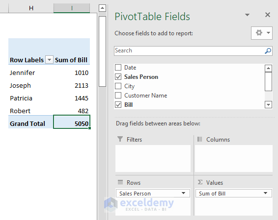
We get the table of bills in terms of each salesperson.

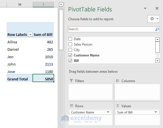
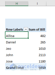
We can also change the data presentation. Select Customer Name instead of the Sales Person and see the changes on the below image.

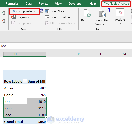
Select three names that start with “J”, those will be in a group.
Go to the PivotTable Analyze tab.
Select the Group Selection option.

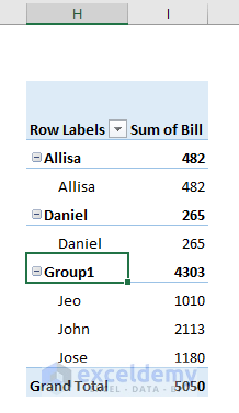
We can see that those cells formed a group named Group1.

We can also apply this grouping in another way.

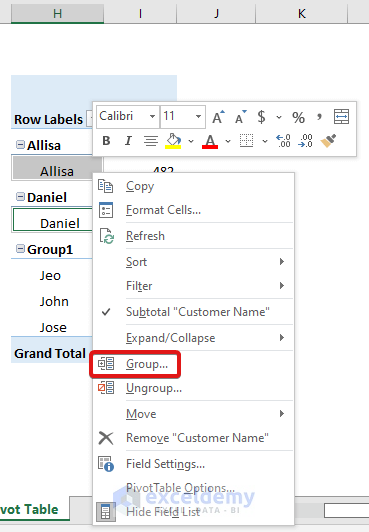
Select the cells.
Right-click on the selection.
Select the Group option.

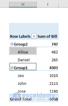
Another group is created named Group2.

Undo Grouping from a Pivot Table

Method 1:

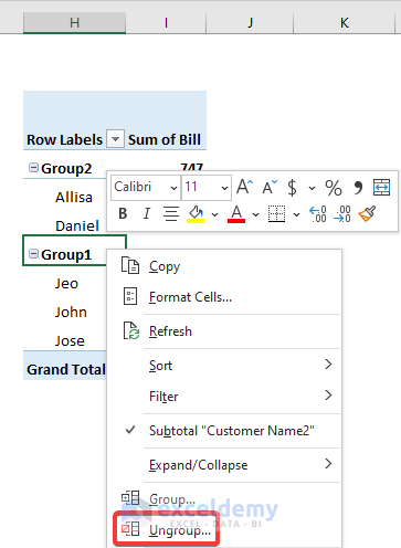
Select any of the groups. We selected Group1.
Right-click on it.
Choose Ungroup from the menu.

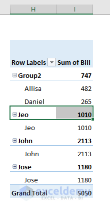
Group1 is removed.

Method 2:

Select Group2.
Go to the PivotTable Analyze tab.
Choose the Ungroup option.

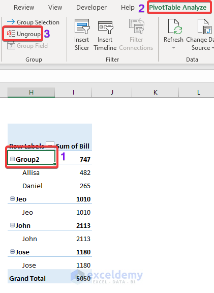
Group 2 is not showing anymore.

Pivot Table for Custom Grouping: 3 Types of Objects

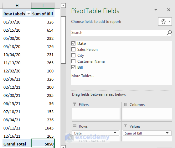
Example 1 – Grouping Dates in a Pivot Table

This grouping is done automatically. We will apply grouping on the below data set, which is formed by data and bill segments.

Case 1.1 – Group Dates Based on Years in a Pivot Table

Steps:

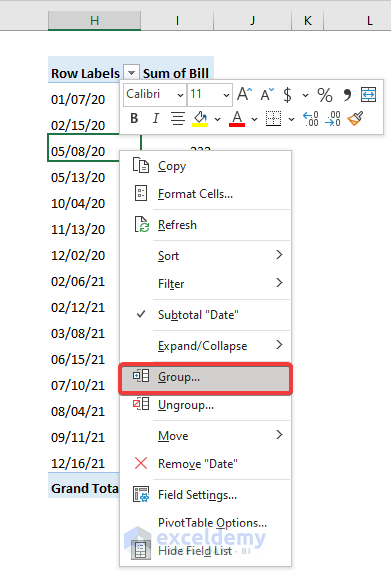
Select any of the cells on the Pivot table.
Right-click and choose Group from the menu.

A dialog box will appear. Tick the boxes of Starting at and Ending at.
Choose Years.

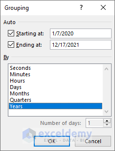
Press OK and see the return.

The Sum of Bill is shown in terms of years only.

Case 1.2 – Group Dates Based on Quarters in a Pivot Table

Steps:

Select any of the cells on the Pivot table.
Right-click and choose Group from the menu.

A dialog box will appear. Tick the boxes of Starting at and Ending at.
Choose Quarters.

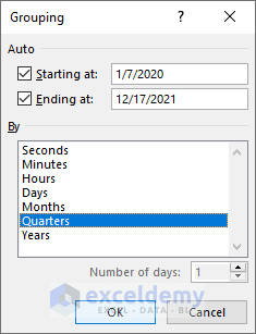
Press OK and see the return.

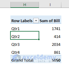
The Sum of Bill is shown in terms of quarters only. However, we cannot identify the quarters with corresponding years.

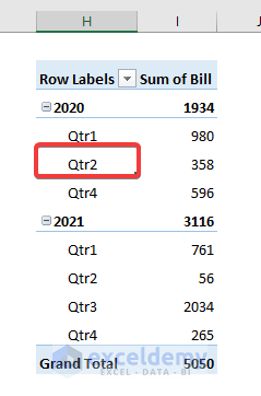
Select both the Quarters and Years from the box.

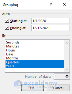
Press OK to see what happens.

Case 1.3 – Group Dates Based on Months in a Pivot Table

Steps:

Select any of the cells on the Pivot table.
Right-click and choose Group from the menu.

A dialog box will appear. Tick the boxes of Starting at and Ending at.
Choose Months.

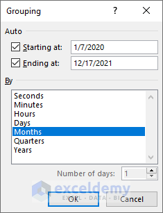
Press OK and see the return.

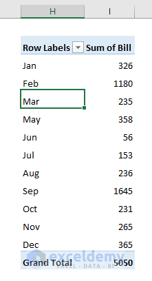
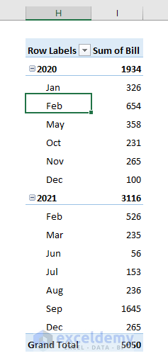
The Sum of Bill is shown in terms of months only.

We can specify the bill of a specific month with a specific year.

Select both the Months and Years from the box.

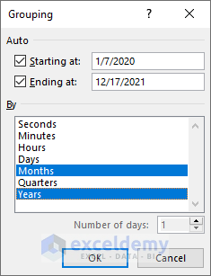
Press OK to see the return.

Case 1.4 – Group Dates Based on the Day in a Pivot Table

Steps:

Select any of the cells on the Pivot table.
Right-click and choose Group from the menu.

A dialog box will appear. Tick the boxes of Starting at and Ending at.
Choose Days.
On the Number of days box, put 7.

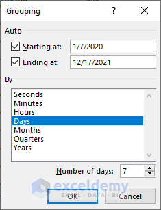
Press OK and see the return.

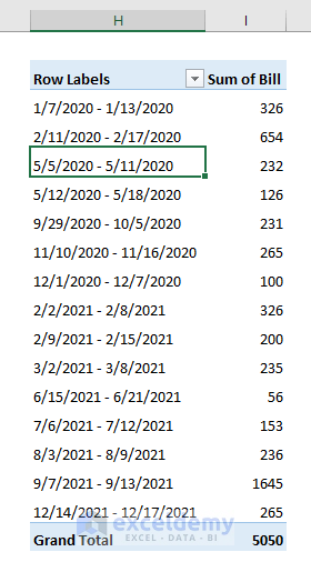
We set the number of days 7 as we want to get the sum for each week. We can also modify this day value and put whatever interval need.

Example 2 – Group Text Items in a Pivot Table

We will show the grouping of text items in the Pivot Table.

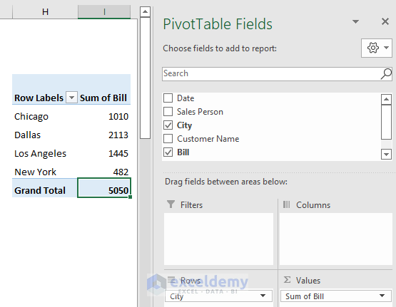
Part 2.1 – Create a Text-based Group in a Pivot Table

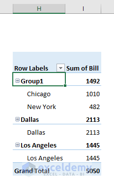
Select Chicago and New York, as both form a group.
Right-click and choose Group from the menu.

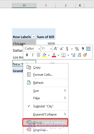
A new group is constructed named Group1.

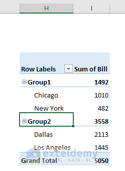
Create Group 2 that consists of Dallas and Los Angeles.

Part 2.2 – Rename a Group in a Pivot Table

Steps:

Select any of the groups. We select Group1.
Press F2.
Put a new name Old_Store.

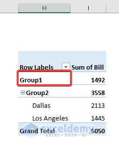
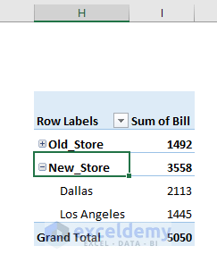
Press Enter and see what happens.

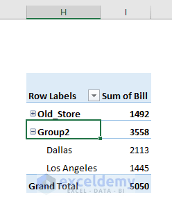
Rename Group2 as New_Store.

Part 2.3 – Change the Cell Format in a Pivot Table

Steps:

Select any of the cells from the value field.
Right-click and choose Value Field Settings.

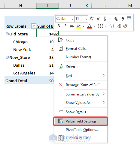
Select Number Format.

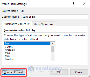
You’ll get the Format Cells dialog.

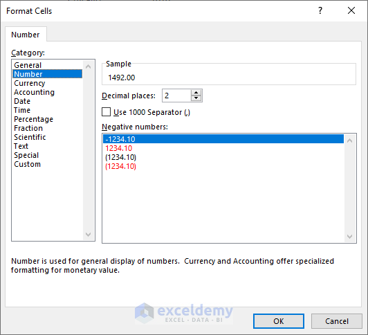
Change the cell format.

Part 2.4 – Some Additional Features of Grouping in a Pivot Table

In this section, we will discuss some additional features of Grouping in the Pivot table.

Go to the Value Field Settings as shown earlier.

From the Summarize value field by box, choose other operations like Max.

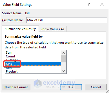
Press OK and see what occurs.

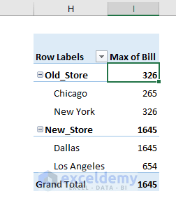
We can also present the value in terms of percentage.

Select Show Values As from the Value Field Settings.

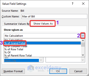
Press OK.

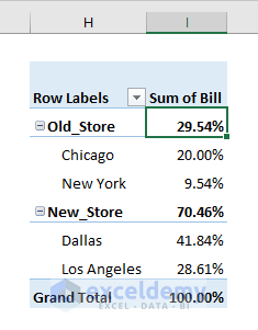
The sum of the bill is represented in percentage.

We can also represent a value in terms of multiple variables.

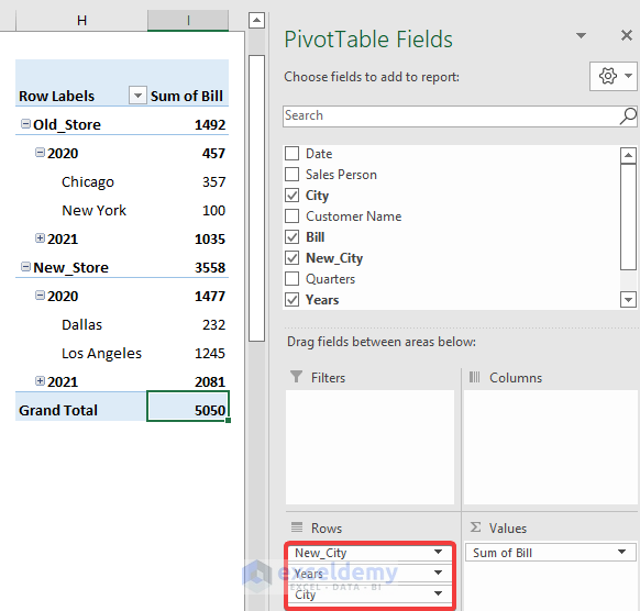
In the first step, values are shown according to the Store, then based on years.

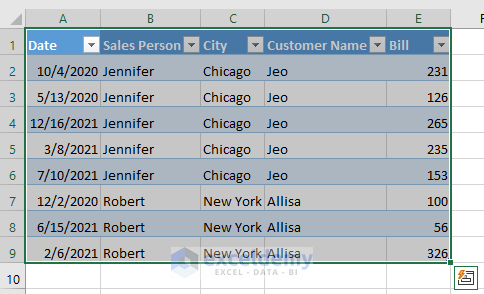
We can also get the details of any specific cell.

Right-click and select Show Details from the menu.

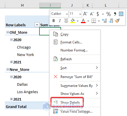
We can see the details of that cell.

Example 3 – Group Numeric Values in Excel

Steps:

We have a Pivot in terms of bills and customer numbers.

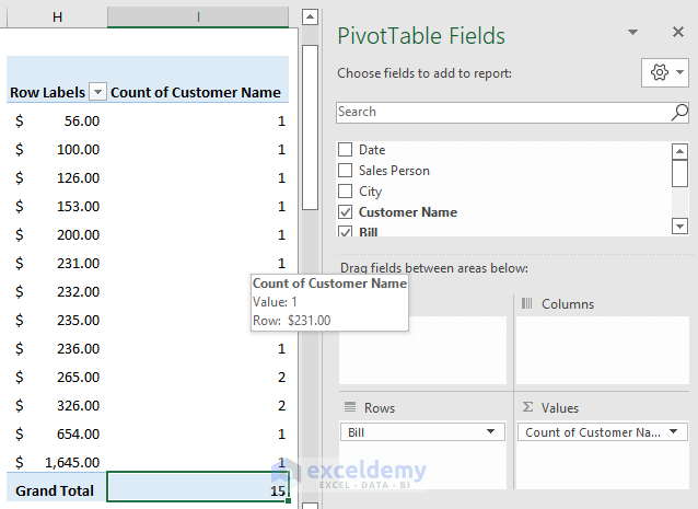
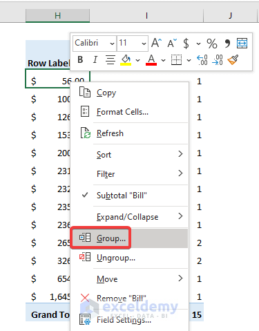
Select any of the cells of the bills.
Right-click and select Group from the menu.

A dialog box will appear. Put the customized values in the boxes.

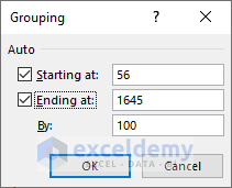
Press OK.

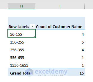
The number of customers is shown in terms of bill amounts.

How to Turn Off Auto-Grouping of Dates in an Excel Pivot Table

This option is available from Excel 2016 to later versions.

Steps:

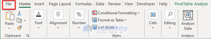
Select File from the main tab.

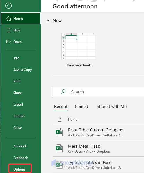
Go to Options.

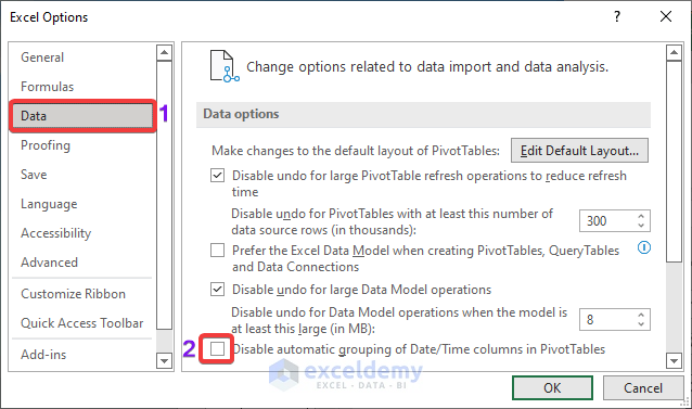
Go to the Data tab.
Check Disable automatic grouping of Date/Time columns in the PivotTables. This option will turn off the auto grouping of date and time.

Note:

This setting change will affect all your Excel workbook files.

Things to Remember

You can also group based on hours, minutes, seconds if the data set contains time arguments.
When creating a Pivot table, be careful about the different PivotTable fields.

Download the Practice Workbook

Pivot Table Custom Grouping.xlsx

Pivot Table Custom Grouping: With 3 Criteria

What Is the Pivot Table in Excel?

What Does Pivot Table Grouping Mean?

How to Create a Pivot Table and Apply Grouping

Undo Grouping from a Pivot Table

Pivot Table for Custom Grouping: 3 Types of Objects

Example 1 – Grouping Dates in a Pivot Table

Case 1.1 – Group Dates Based on Years in a Pivot Table

Case 1.2 – Group Dates Based on Quarters in a Pivot Table

Case 1.3 – Group Dates Based on Months in a Pivot Table

Case 1.4 – Group Dates Based on the Day in a Pivot Table

Example 2 – Group Text Items in a Pivot Table

Part 2.1 – Create a Text-based Group in a Pivot Table

Part 2.2 – Rename a Group in a Pivot Table

Part 2.3 – Change the Cell Format in a Pivot Table

Part 2.4 – Some Additional Features of Grouping in a Pivot Table

Example 3 – Group Numeric Values in Excel

How to Turn Off Auto-Grouping of Dates in an Excel Pivot Table

Things to Remember

Further Readings

Leave a reply Cancel reply