Excel Pivot Table Example (11 Different Case)

What Is a Pivot Table in Excel?

A Pivot Table is an amazing data analysis tool of Microsoft Excel. It can analyze data according to our desired requirements. It can summarize data in several types of categories and subcategories. The Pivot Table also has all the features of a conventional Excel table.

How to Create a Pivot Table in Excel

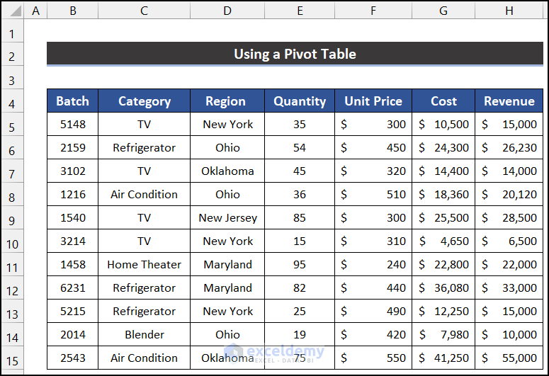
We are going to use a dataset that has 11 shipment information of an electric supplier. Our dataset is in the range of cells B5:H15.

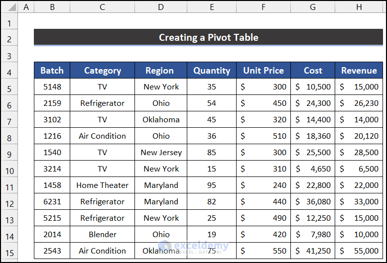
Steps:

• Select the range of cells B4:H15.
• In the Inset tab, click on the drop-down arrow of the PivotTable option from the Table group and select the From Table/Range option.

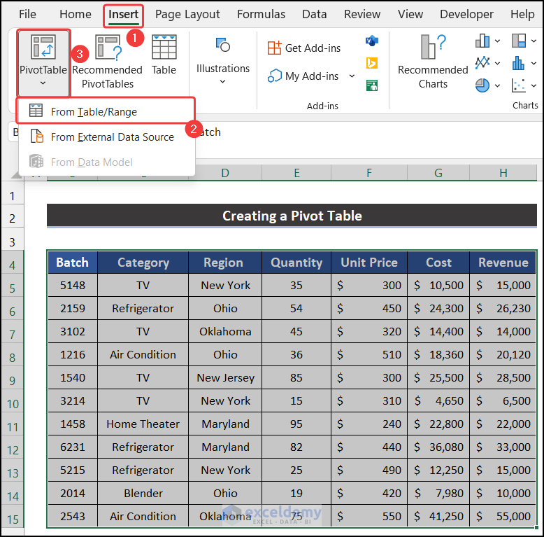
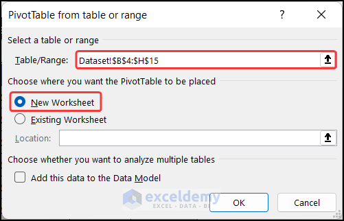
• A small dialog box called Pivot Table from table or range will appear.
• Set the destination of the Pivot Table. For our dataset, we chose the New worksheet option.
• Click OK.

• A new worksheet will be created, and the Pivot Table will appear in front of you.

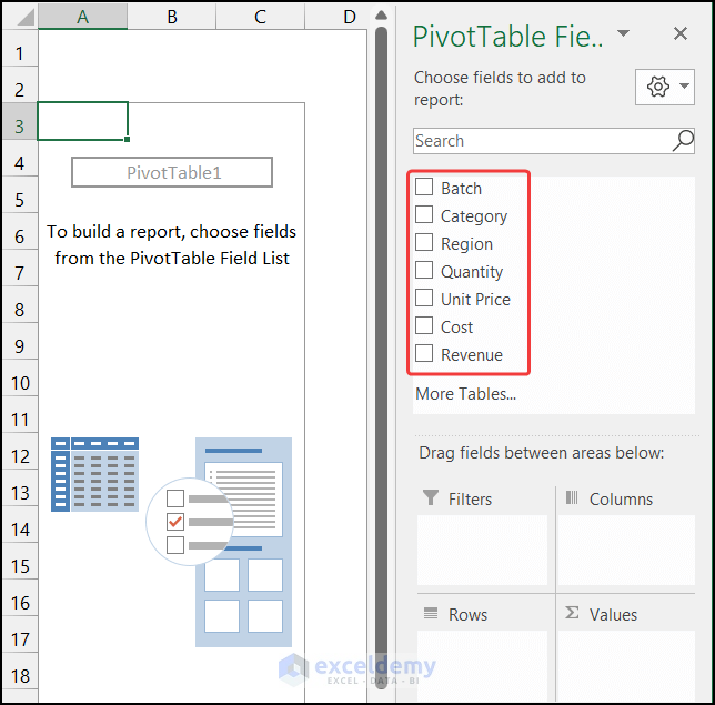
• Input the fields in the four areas of the Pivot Table to get the value in it.

How Does a Pivot Table Work?

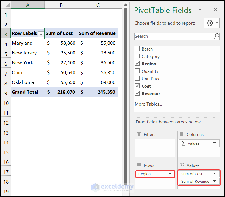
In the Pivot Table Field window, there are four areas. They are Filters, Columns, Rows, and Values. Above them, we have the field name list where all the column headings of our main table remain listed. We can input a field in those areas once to display the corresponding data in our Pivot Table. Insertion of a field in the different areas results in different outputs in our Pivot Table.

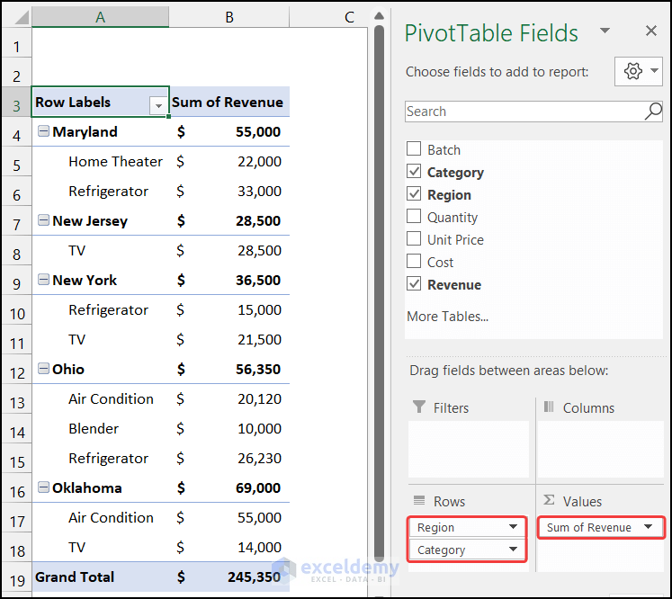
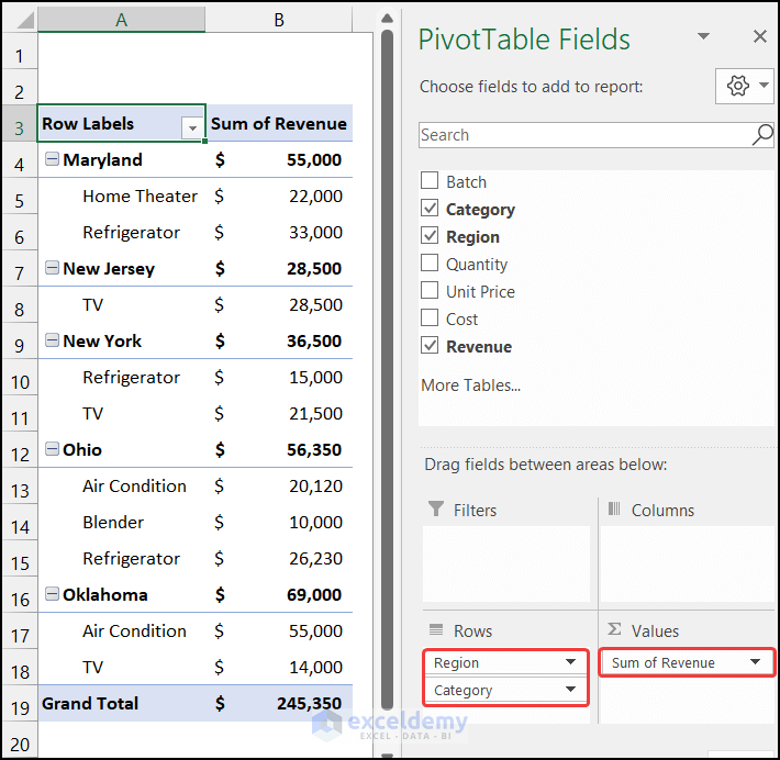
If we placed the Region and Category in the Rows area and the Revenue field in the Value area, the Pivot Table shows us a result like the image shown below.

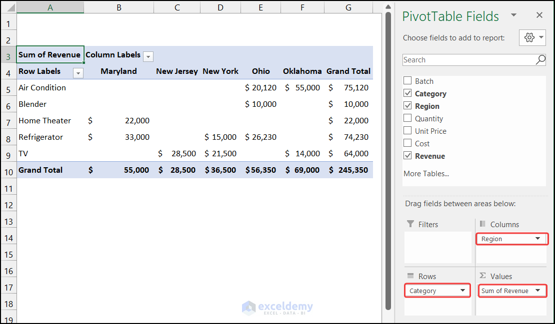
If we just take any of a field from the Rows area to the Columns area, we will notice the output will be completely changed and the Pivot Table will display a new output.

Excel Pivot Tables: 11 Examples

Consider a dataset of 11 deliveries of an electric product supplier. The information on every shipment is in the range of cells B5:H15. We will show you several types of Pivot Tables.

Example 1 – Inserting the Fields into Analyze Data in Pivot Table

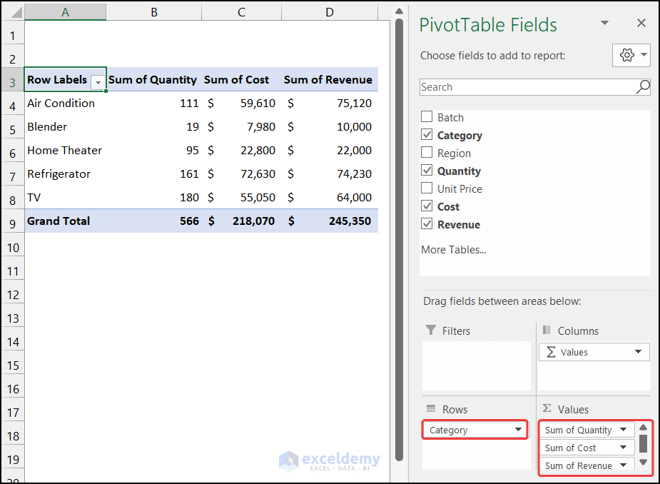
We will add the fields Quantity, Cost, and Revenue in our Pivot Table against the Category.

Steps:

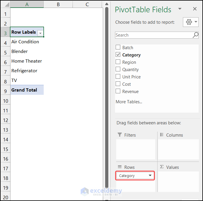
• As we want to display all of those data with respect to the Category field, at first, we will place the Category field.
• Drag the Category field from the field list into the Rows area.

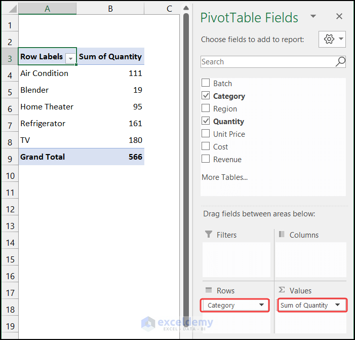
• Drag the Quantity field in the Value area. The value of the quantity will be shown in column B.

• Input the Cost and Revenue field in the Value area.
• You will get all the fields in the Pivot Table.

Read More: A Pivot Table Example in Excel with Real Data

Example 2 – Nesting Multiple Fields in a Single Section

We are going to show the nesting fields in a single area. In our Pivot Table, we have the Revenue value with the Category field.

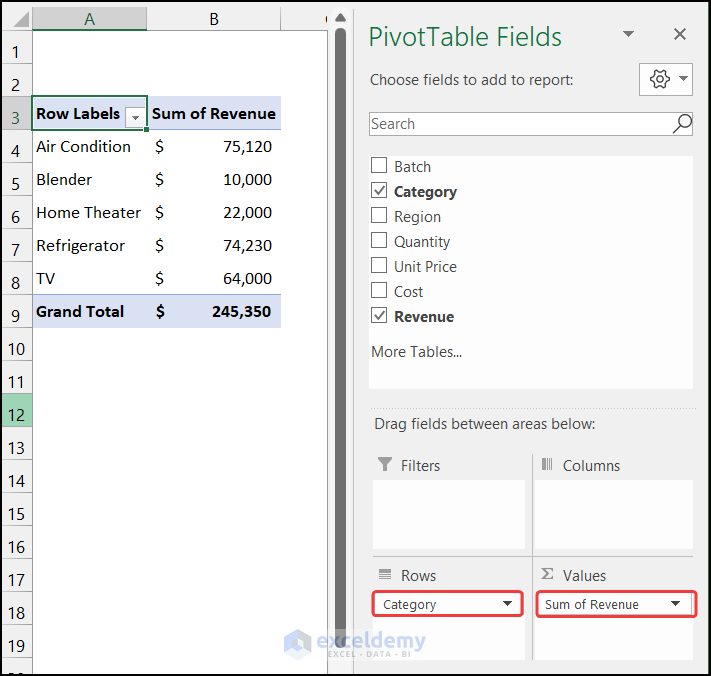
We will input the Region field in the Rows area to form a nested filed situation.

Steps:

• Drag the Region field from the field name list into the Rows area above the Category field.
• You will see that the region name will show first, and inside every region, the corresponding category will display.

Example 3 – Placing a Slicer for a Pivot Table

Steps:

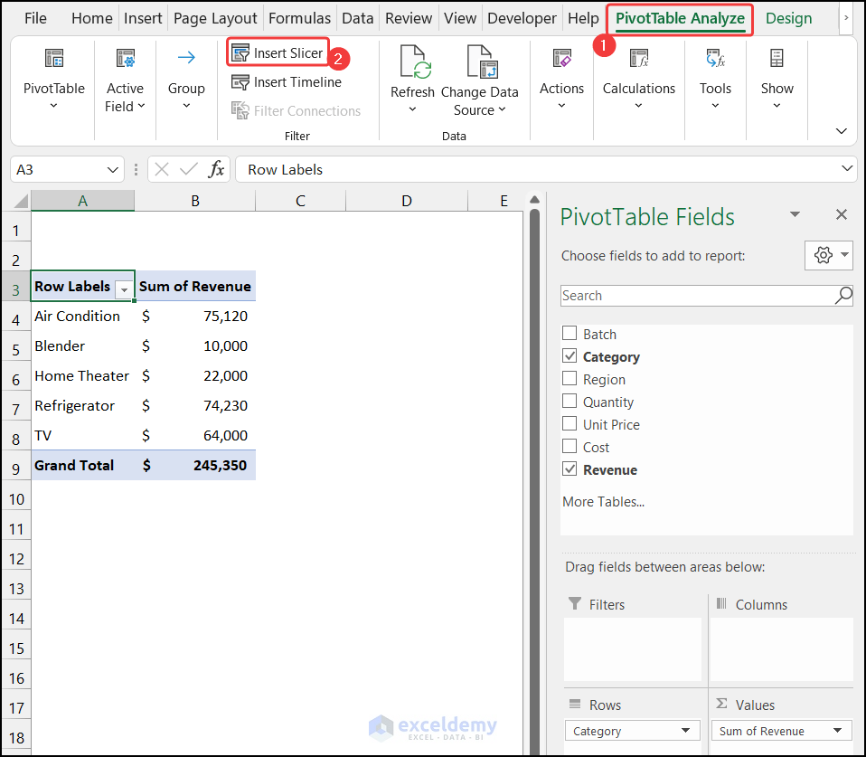
• In the Pivot Table Analyze tab, select the Insert Slicer option from the Filter group.

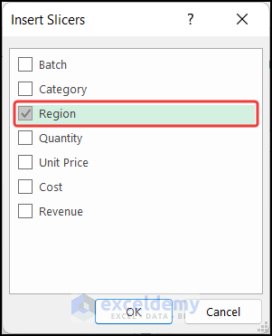
• A small dialog box titled Insert Slicers will appear.
• Select the field name for which you want to insert the Slicer. We checked the Region field.
• Click OK.

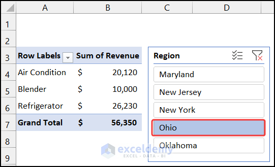
• A Region Slicer will appear.

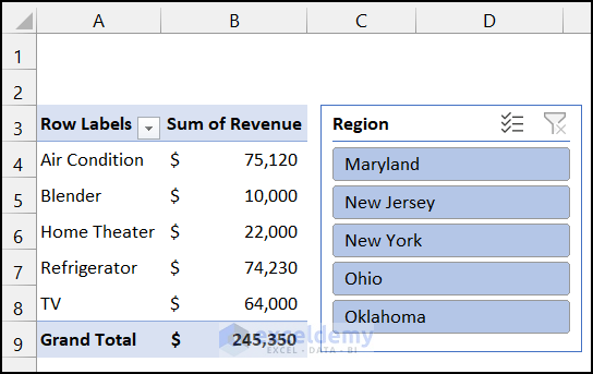
• Select any of the regions, and you will see the corresponding category in the Pivot Table.

Example 4 – Sorting Data

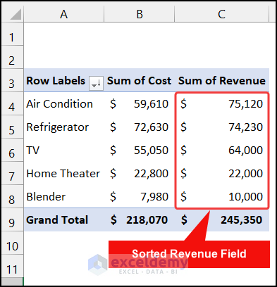
We want to sort our Pivot Table from the highest revenue to the lowest revenue.

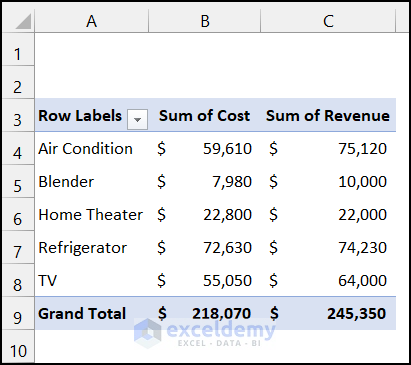
Steps:

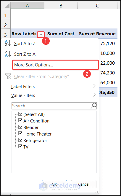
• Click on the drop-down arrow located at the bottom corner of the Row Labels.
• Select the More Sort Options option from the Context Menu.

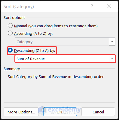
• The Sort (Category) dialog box will appear.
• Choose the Descending (Z to A) by filed and change the filed option Category to Sum of Revenue.
• Click OK.

• The highest revenue cell is displayed at the top and the lowest one at the bottom.

Example 5 – Filtering Data According to a Requirement

Steps:

• Click on the drop-down arrow allocated at the bottom corner of the Row Labels.

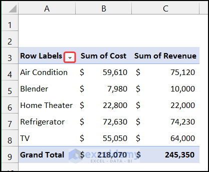
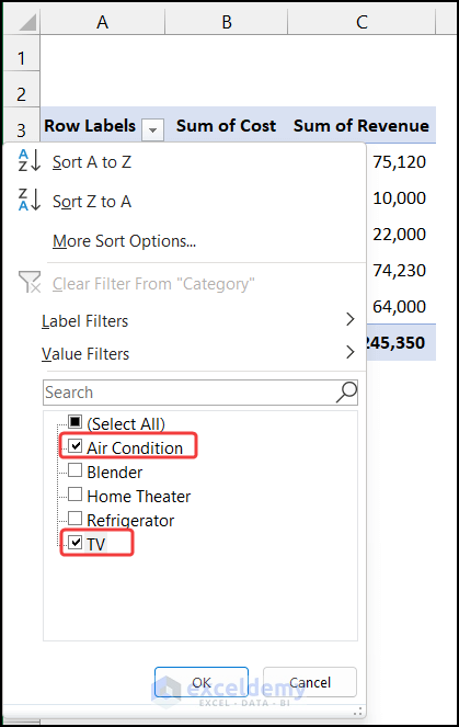
• The Context Menu will appear.
• Check those entities that you want to keep. We checked only for TV and Air Condition to see their data.
• Click OK.

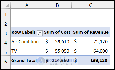
• You will get the data of only those two items.

Example 6 – Updating Data in a Pivot Table

We will add a new data series to our dataset. The range of our dataset is in the range of cells B5:B16.

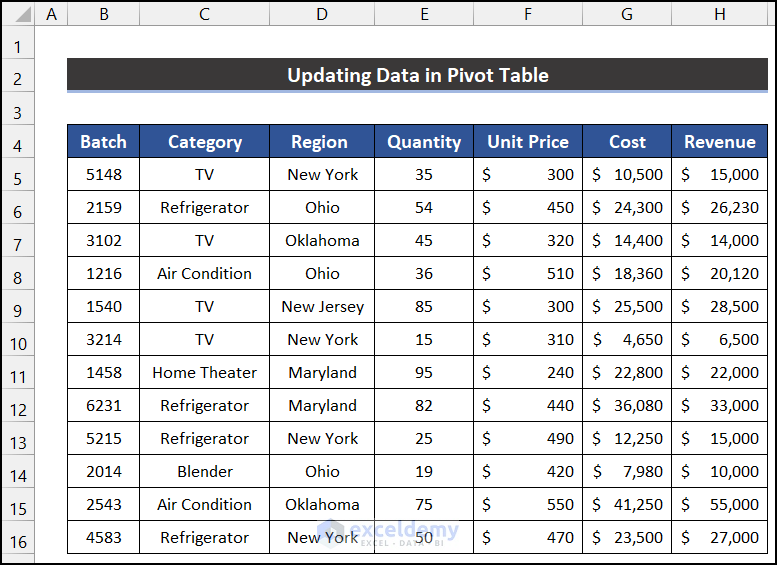
Steps:

• In the Pivot Table Analyze tab, click on the drop-down arrow of the Change Data Source and select the Change Data Source option from the Data group.

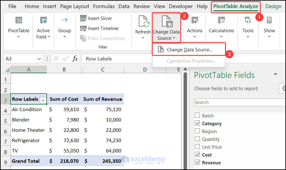
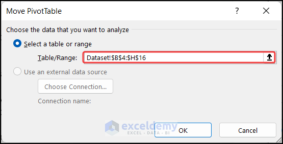
• The Change Pivot Table Data Source will appear.
• Select the new data range in the Table/Range field.
• Click OK.

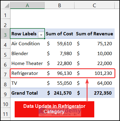
• The Pivot Table is updated with the new data.

Example 7 – Getting the Top 3 Values from a Table

Steps:

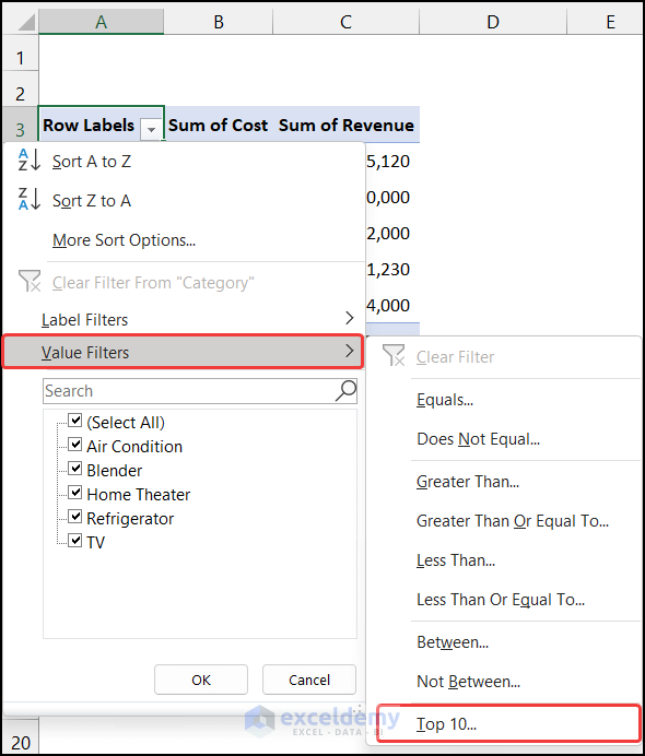
• Click on the drop-down arrow allocated at the bottom corner of the Row Labels.

• The Context Menu will appear.
• Select the Top 10 option from the Value Filters group.

• Another dialog box called Top 10 Filter (Category) will appear.
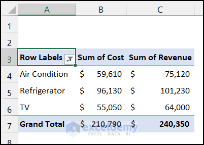
• To get the top 3, reduce the number from 10 to 3.
• Set the last field as the Sum of Cost.
• Click OK.

• You will get three items.

Example 8 – Data Grouping with a Pivot Table

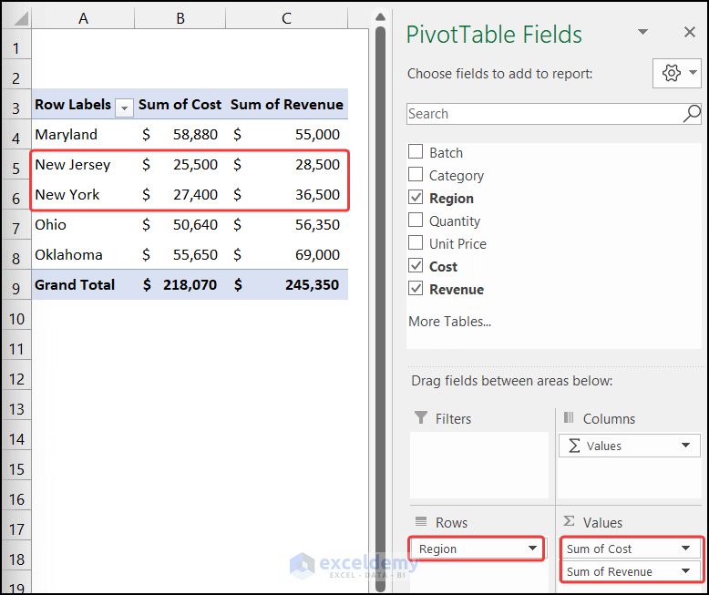
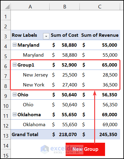
We keep the Region field in the Rows area. We know that New York and New Jersey are two neighboring states. So, we want to keep them in a group.

Steps:

• Select the range of cells A5:A6.
• Right-click and select the Group option.

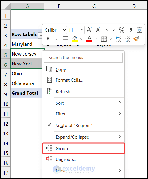
• Both regions will be assigned to a new group and the others will be shown as an individual group.

Read More: Pivot Table Test for Interview

Example 9 – Analyzing Data with a Pivot Chart

Steps:

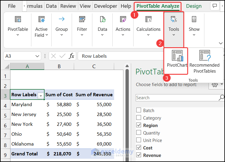
• In the Pivot Table Analyze tab, select the Pivot Chart option from the Tools group.

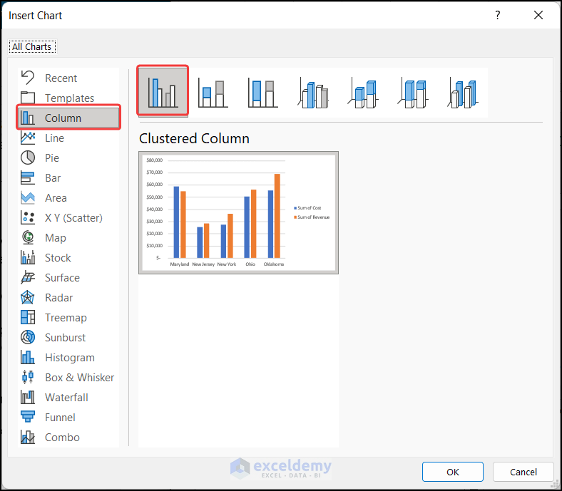
• The Insert Chart dialog box will appear.
• Choose a chart. We chose the Clustered Column chart for a better comparison of our dataset.
• Click OK.

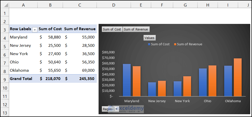
• The chart will appear on the sheet.
• Modify the chart according to your requirements and add necessary items from the Chart Elements icon.

Read More: Excel Data for Pivot Table Practice

How to Refresh a Pivot Table

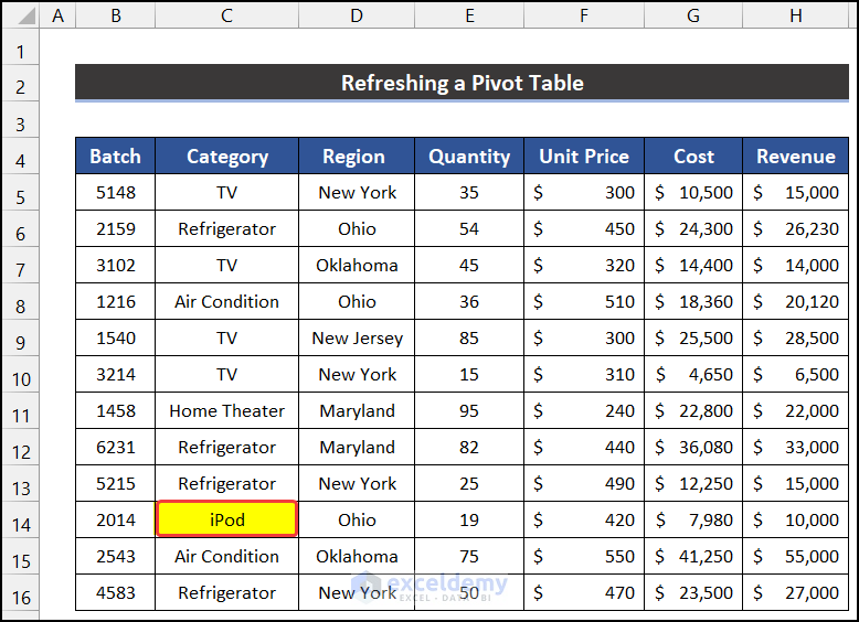
We changed a category name from Blander to iPod, but we need to update the pivot table.

Steps:

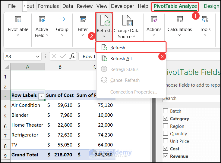
• Go to the Pivot Table Analyze tab.
• Select Refresh and choose the Refresh option from the Data group.

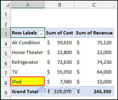
• Blender will be replaced with iPod.

Read More: What Is the Use of Pivot Table in Excel

How to Move a Pivot Table to a New Location

Steps:

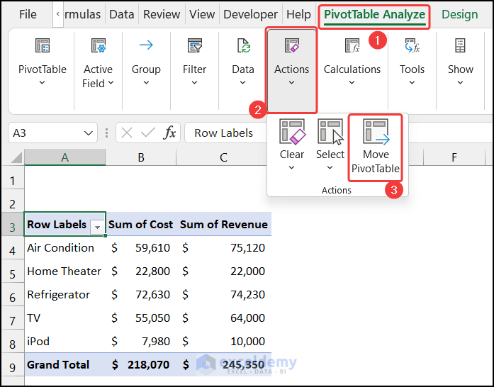
• Go to the Pivot Table Analyze tab.
• Click on the Move Pivot Table from the Action group.

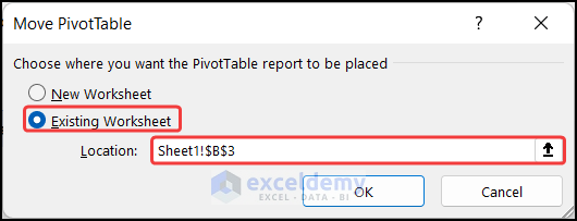
• The Move Pivot Table dialog box will appear.
• Set the destination of your Pivot Table. We want to move one column to the right, so we chose the Existing Worksheet option and selected cell B3 as a cell reference.
• Click OK.

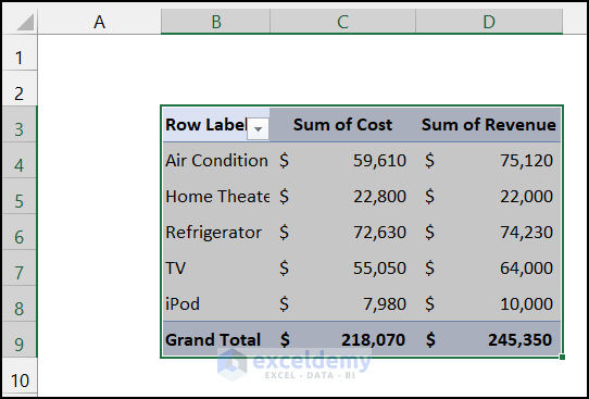
• The whole Pivot Table will shift one column.

How to Remove a Pivot Table

Steps:

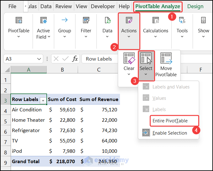
• In the Pivot Table Analyze tab, click on the drop-down arrow of Select, then choose the Entire Pivot Table option from the Action group.

• You will get the complete table selected.

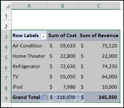
• Press the Delete key from your keyboard.
• The Pivot Table will disappear from the sheet.

Download the Practice Workbook

<< Go Back to What is Pivot Table in Excel | Pivot Table in Excel | Learn Excel