How to Reference Cell by Row and Column Number in Excel (4 Methods)

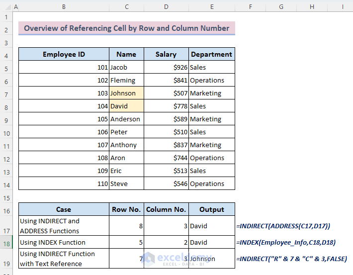
This article will show you four ways to reference a cell by row and column number in Excel with sharp steps and vivid illustrations. In the following overview image, you’ll see different methods to reference cell by row and column number in Excel.

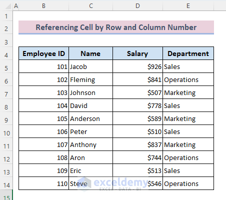
All of the below methods use the following dataset:

Method 1-  Use INDIRECT and ADDRESS Functions to Reference Cell by Row and Column Number

Steps:

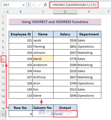
• Highlight Cell D17 and type the following formula in it-

• Hit the Enter button to get the output.

⏬ Formula Breakdown:

➥ ADDRESS(B17,C17))

The ADDRESS function will return the default cell reference for row number 8 and column number 3. So it will return as-

“$C$8”

➥ INDIRECT(ADDRESS(B17,C17))

The INDIRECT function will return the value of that cell according to the cell reference:

“David”

Read More: How to Display Text from Another Cell in Excel

Method 2 – Use the INDEX Function to Reference Cell by Row and Column Number

Steps:

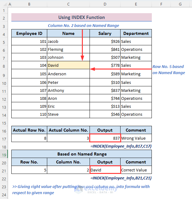
• As we put the below formula in Cell D17 we’re getting the wrong result as we’ve put the actual row and column number of our Excel sheet into the formula:

• Here, the Employee_Info part is the range of our dataset, from where the INDEX function will search for the value. And B17 and C17 is denoting the actual row number 8 and column number 3 of your Excel sheet.

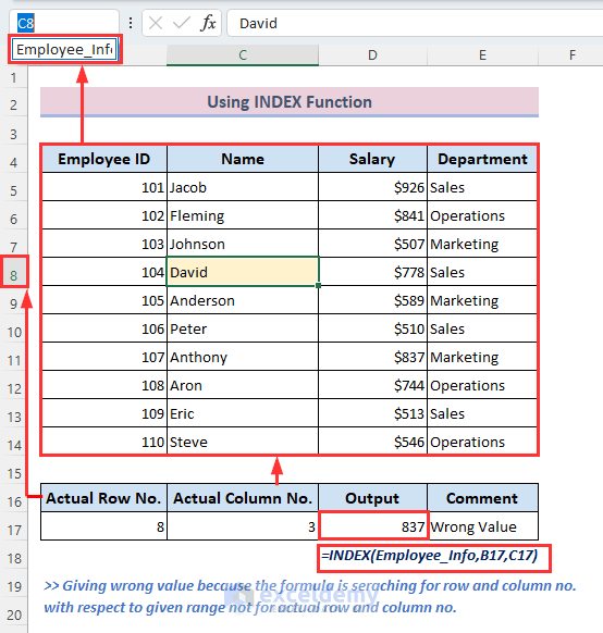
• To fix this, enter the following formula in D21 to get the correct result for Employee_Info–

• B21 and C21 denote the row number 5 and column number 2 based on the given range Employee_Info.

Read More: How to Reference Text in Another Cell in Excel

Method 3 – Use Text Reference Within the INDIRECT Function to Reference Cell by Row and Column Number

Steps:

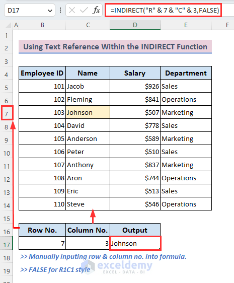
• In Cell D17, type the following formula and hit the Enter button for the result–

• This function will search for the value from row number 7 and column number 3 which is Johnson and brings it here. We put FALSE because we are using the R1C1 style here.

Read More: How to Use Variable Row Number as Cell Reference in Excel

Method 4 – Reference Cell by Row and Column Number Applying User Defined Function

Steps:

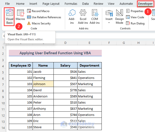
• Go to the Developer tab and click on the Visual Basic menu to open the Visual Basic Editor.

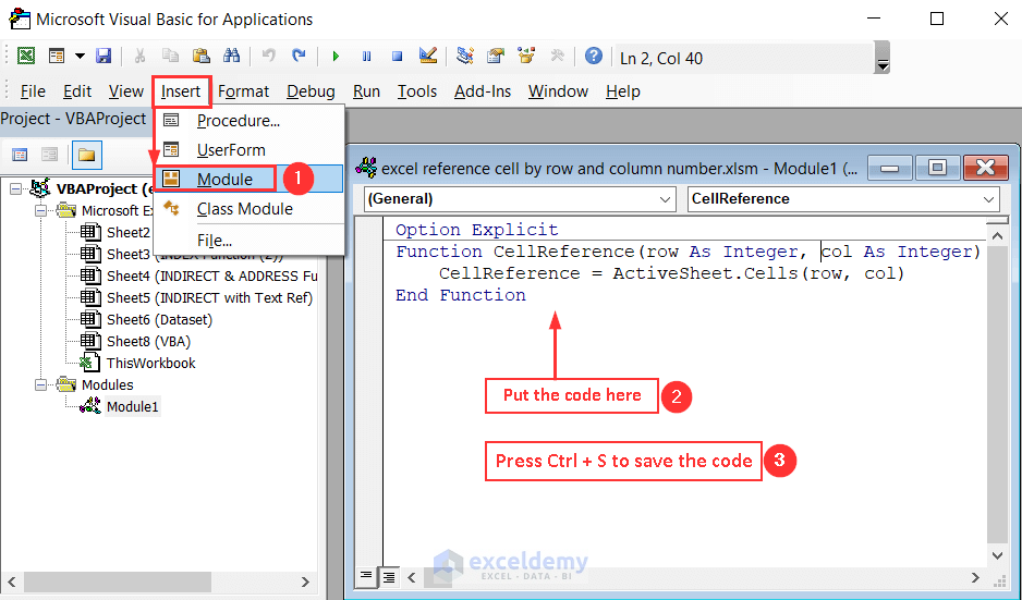
• Select Module under the Insert tab.
• Insert the following VBA code:

Option Explicit
Function CellReference(row As Integer, col As Integer)
    CellReference = ActiveSheet.Cells(row, col)
End Function

• Save the code by pressing Ctrl + S together.
• Minimize the VBA window and go back to your sheet.

• The formula is ready to use. However, you have to give the row number and column number and it will return the value according to that reference.
• To get the value from Cell C7, type the following formula in Cell D17–

• Press the Enter button to finish.
• This delivers the correct value – Johnson.

Read More: How to Find and Replace Cell Reference in Excel Formula

Download Practice Workbook

You can download the free Excel template from here and practice on your own.

Related Articles

• How to Use Cell Value as Worksheet Name in Formula Reference in Excel
• How to Use OFFSET for Cell Reference in Excel
• How to Reference a Cell from a Different Worksheet in Excel
• How to Reference Cell in Another Sheet Dynamically in Excel
• Excel VBA Examples with Cell Reference by Row and Column Number
• Excel VBA: Cell Reference in Another Sheet 

<< Go Back to Cell Reference in Excel | Excel Formulas | Learn Excel