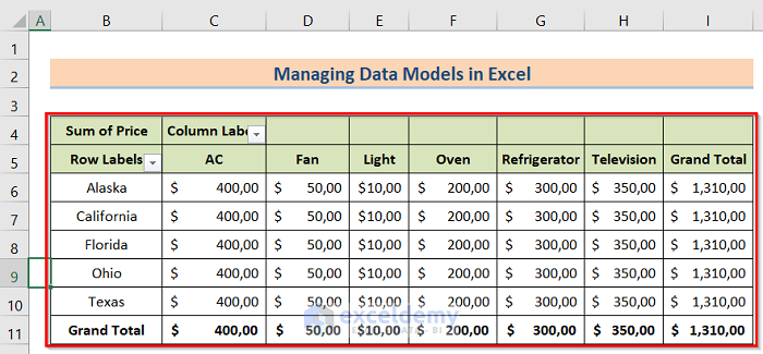
What Is a Reference of Data Model in Excel?
Data model referencing means taking value from the pivot table to another cell. Sometimes you need to take some specific data from the pivot table. In that case, referencing is essential. The Pivot table helps you narrow down a large dataset and establish a relationship between data points. It recognizes the dataset metrics and dimensions and provides a meaningful summary of it. After creating the pivot table, you may have needed to refer to another cell or a new worksheet. In that case, you can use the GETPIVOTDATA function. You can use direct cell reference, but if you alter the Pivot Table format, the cell will show an error.
How to Use the Reference of Data Model in Excel Formula: Step-by-Step Procedures
Step 1 – Arranging the Dataset
We have Month in Column B, Year in Column C, Income in Column D, and Expenses in Column E.
- Insert the values as needed.

Step 2 – Creating a Pivot Table
- Select the dataset.
- Go to Insert and select PivotTable.
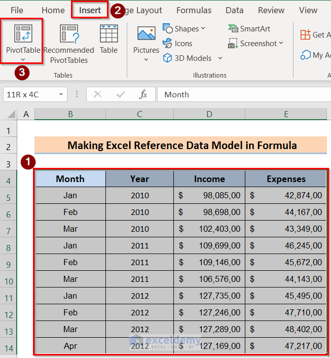
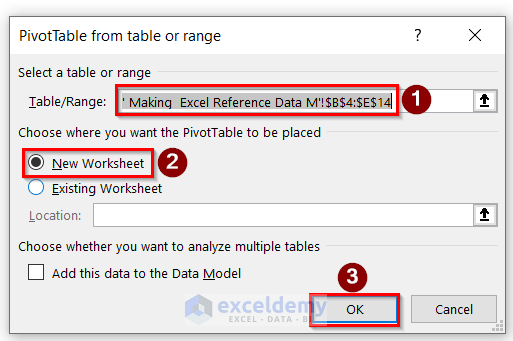
- In the ‘PivotTable from table or range’ dialog box, choose the desired range in the Select a table or range option.
- Check the New Worksheet option and click on OK.
- On the right side of your Excel window, you will find the PivotTable Fields. Check all the columns.
- Drag the columns to the respective fields.
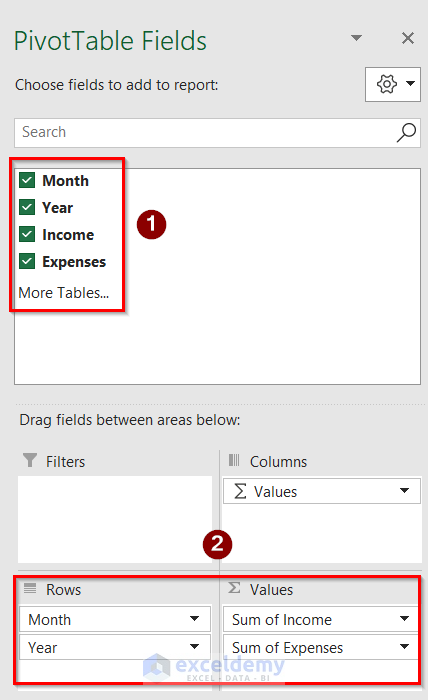
- You will get the desired result.
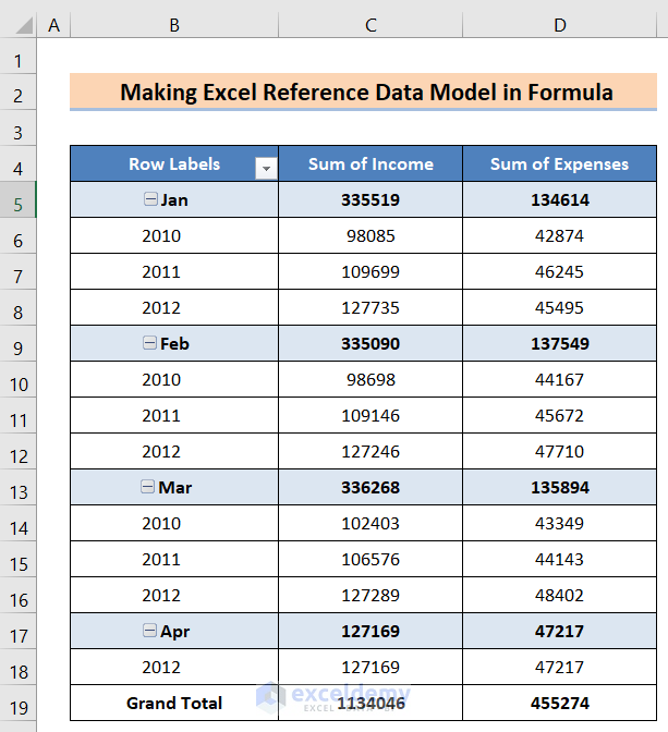
Step 3 – Inserting the Formula to Show the Final Outcome
- Insert the following formula in the F5 cell.
=GETPIVOTDATA("Sum of Expenses",$B$4,"Month","Jan")/GETPIVOTDATA("Sum of Income",$B$4,"Month","Jan")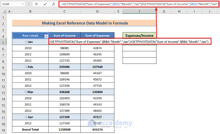
- Hit Enter.
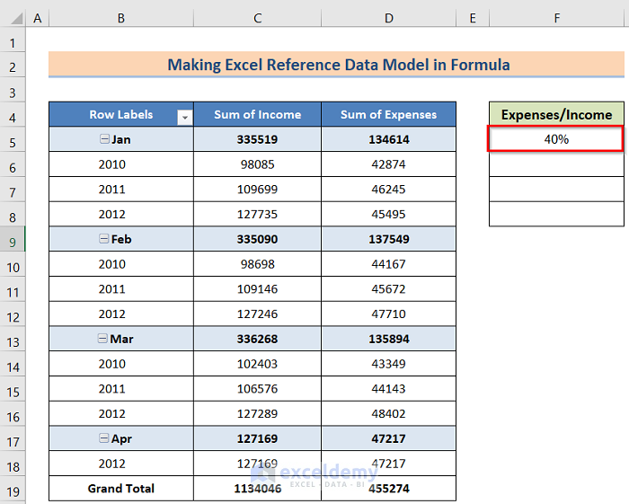
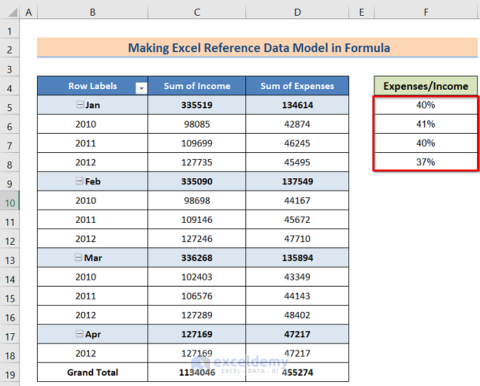
- You must manually input formulas in every cell and change them accordingly.
How to Create Excel Data Model Relationships
Steps:
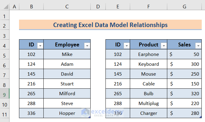
- Arrange the data tables like the image below.
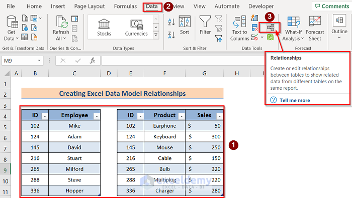
- Go to Data then to Data Tools, and select Relationships.
- In the Create Relationship dialog box, select the Table, Related Table, Column, and Related Column accordingly and then press OK.

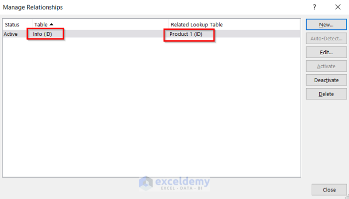
- You will get the result in the Manage Relationships like the image below.
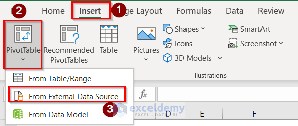
- Go to Insert, then to PivotTable, and choose From External Data Source.
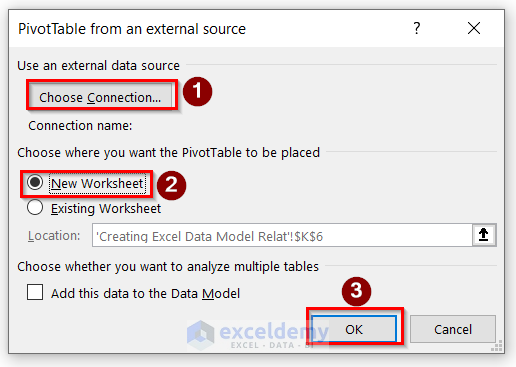
- In the PivotTable from an External source dialog box, select the Choose Connection.
- Select the New Worksheet option and click on the OK button.
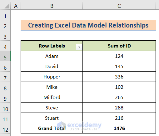
- You will get the desired result.
Read More: How to Add Table to Data Model in Excel
How to Manage Data Models in Excel
Steps:
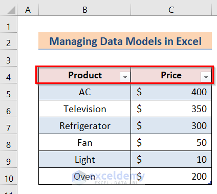
- We need to prepare a compatible dataset. We have Product in Column B and Price in Column C.
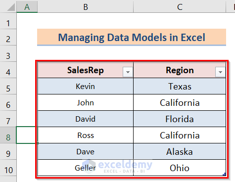
- Create another table where we have SalesRep in Column B and Region in Column C.
- Go to Insert then select PivotTable, and choose From Data Model.
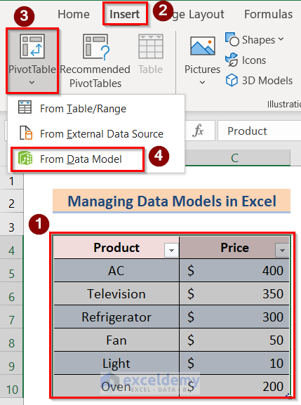
- You will find the PivotTable Fields and press the desired option you want to show in your table.
- Select the Columns, Rows, and Values accordingly.
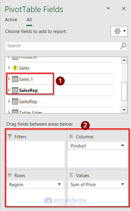
- Here’s our result.
Read More: How to Update Data Model in Excel
Excel Data Model vs. Power Query
In this case, our goal is to compare Excel Data Model with Power Query. A data modeling tool called Power Pivot enables you to build data models, define relationships, and do computations. With Power Pivot, you can deal with enormous data sets, establish intricate relationships, and produce sophisticated or simple calculations all inside the comfortable confines of Excel.
Sometimes, you need to combine two tables in Excel. You can do it manually but that takes a lot of valuable time. Instead of doing this manually, you need to utilize a power query for that purpose. Power query initially set up a connection between two tables in Excel. After that, It merges the tables effectively. Moreover, we can also split columns using a power query. Splitting columns by using the power query is an easy task. In addition, the Power Query in Excel transforms rows into columns very handy.
Read More: Excel Data Model vs. Power Query: Main Dissimilarities to Know
Get Data from Data Model in Excel
Steps:
- Prepare a dataset like an image below.
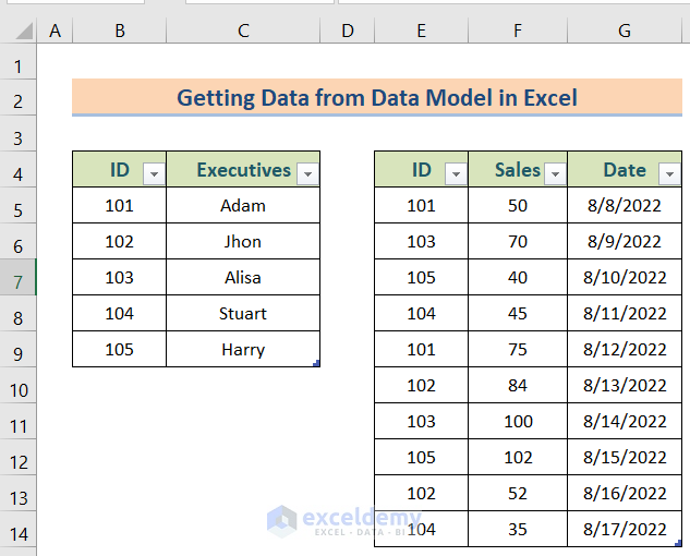
- Insert a PivotTable and choose From External Data Source.
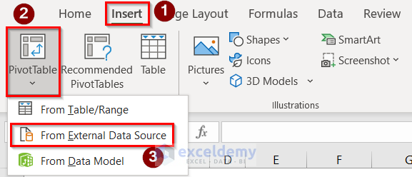
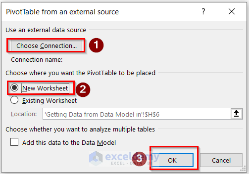
- In the PivotTable from an External source dialog box, select Choose Connection.
- Check New Worksheet and click on the OK button.
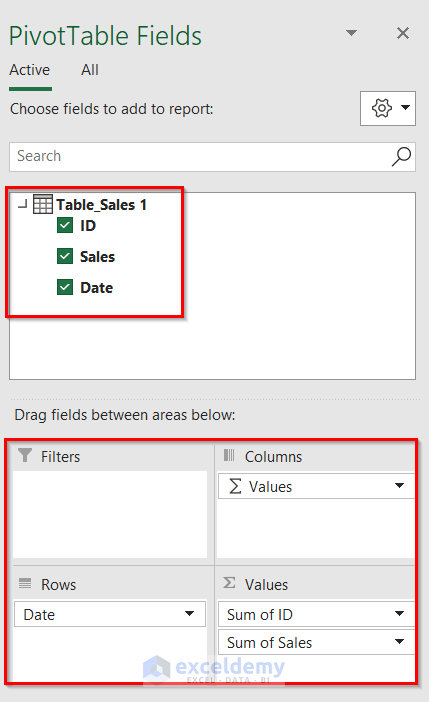
- On the right side of your Excel window, you will find the PivotTable Fields. Press the desired option you want to show in your table.
- Select the Columns, Rows, and Values, accordingly.
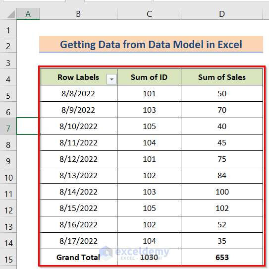
- Here’s our result.
Read More: How to Get Data from Data Model in Excel
Download the Practice Workbook
Related Articles
<< Go Back to Data Model in Excel | Learn Excel
Get FREE Advanced Excel Exercises with Solutions!
