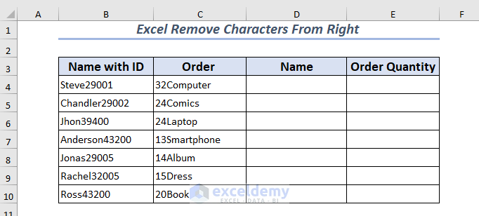
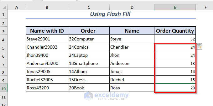
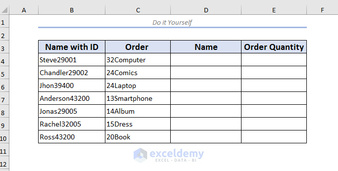
Consider the following dataset. The table represents the order information of different users. The columns are Name with ID, Order, Name, and Order Quantity. We’ll separate the numbers and the text from the first two columns and put them in new ones.
Excel Remove Characters From the Right: 5 ways
Method 1 – Using the LEFT Function to Remove Characters from the Right
- Select the cell where you want to place your new value after removing the last character. We chose D4.
- Use the following formula in the Formula Bar:
=LEFT(B4,LEN(B4)-1)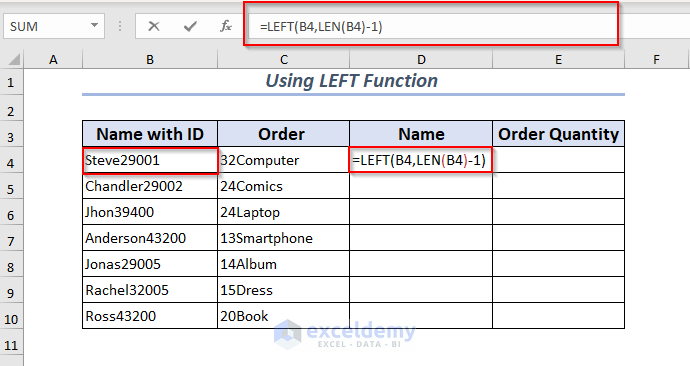
- Press Enter.
The last character from the selected B4 cell will be removed.
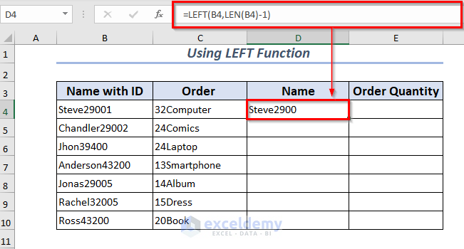
Only removing a single character doesn’t match the context of our example, so let’s remove multiple characters.
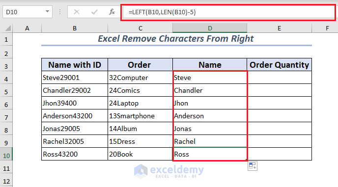
- Use this formula to remove the last five characters from cell B4:
=LEFT(B4,LEN(B4)-5)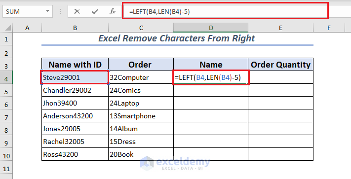
- Press Enter.
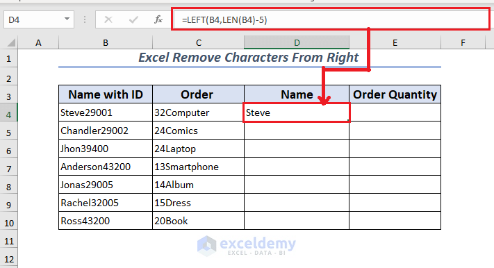
- Apply the Fill Handle to AutoFit the formula for the rest of the cells.
Method 2 – Use VALUE and LEFT Function for Numeric Values
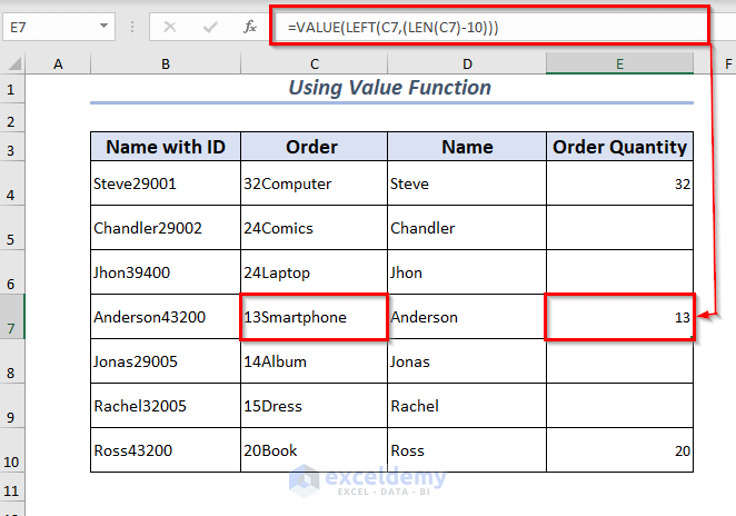
Let’s extract the order quantity (the number at the start of the Order value).
- Select the cell where you want to place your new value after removing the characters from the right. We selected the B4 cell.
- Use the following formula.
=VALUE(LEFT(C4,(LEN(C4)-8)))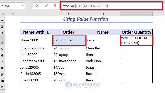
- Press Enter. The string characters of the C4 cell will be removed from the right. You will only see the numeric values in Number format in the Order Quantity column.
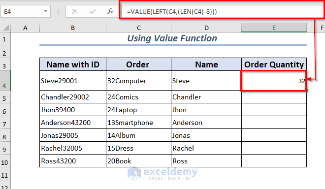
However, the formula removes eight characters regardless of the length of the string, so it won’t work for all cells in the example.
Method 3 – Remove Characters From the Right using VBA
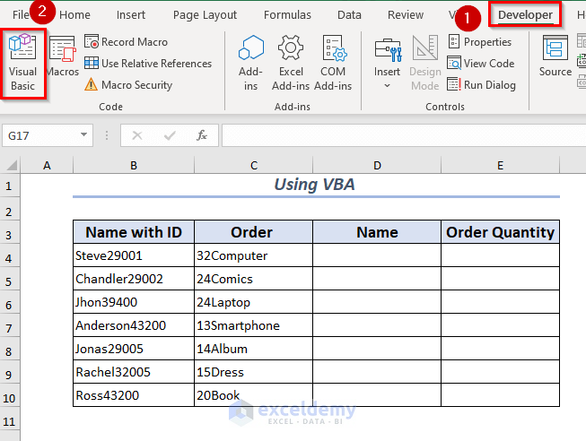
- Go to the Developer tab and select Visual Basic. You also can use Alt + F11.
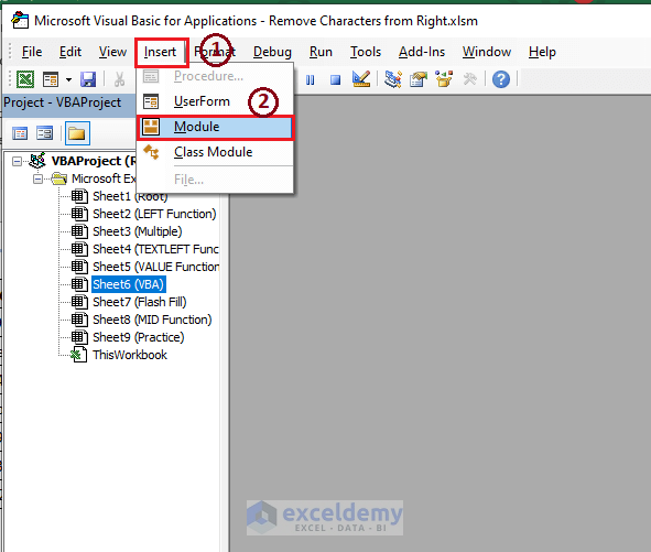
- A new window for Microsoft Visual Basic for Applications will appear. Open the Insert tab and select Module.
- This opens a new Module.
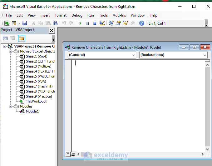
- Insert the following code for the function named RemoveRightCharacter in the module.
Function RemoveRightCharacter(str As String, cnt_chars As Long)
RemoveRightCharacter = Left(str, Len(str) - cnt_chars)
End Function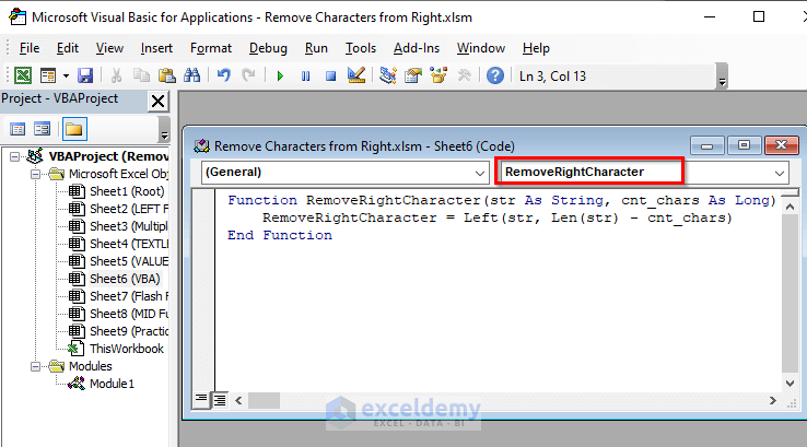
- Save the code and go back to the worksheet.
- Select a cell where you want to keep your new value after removing the character from the right.
- Use the following formula:
=RemoveRightCharacter(B4,5)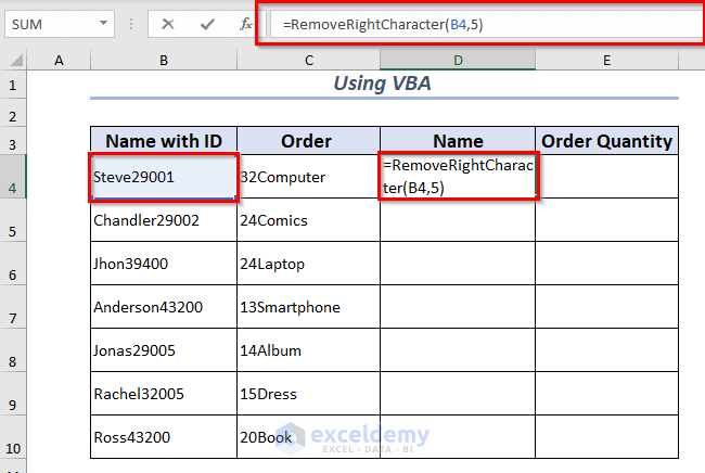
- Press Enter.
- Based on the arguments, the function removes 5 characters from cell B4 and copies the rest into the result cell.
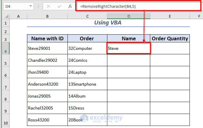
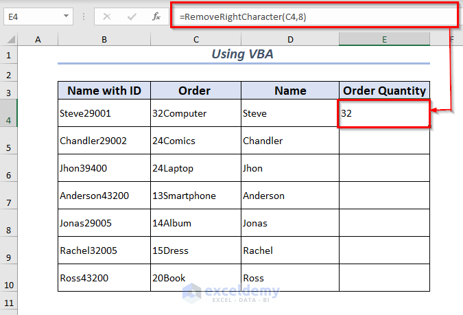
- To apply the formula to remove the string name from the order value, use the following function in E4.
=RemoveRightCharacter(C4,8)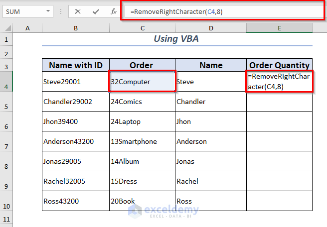
- Press Enter.
Method 4 – Remove the Right Character Using Flash Fill
- Create a pattern example to use Flash Fill.
- We provided the first example, Steve, by manually typing it.
- Select the example value and open the Data tab, then select Flash Fill.
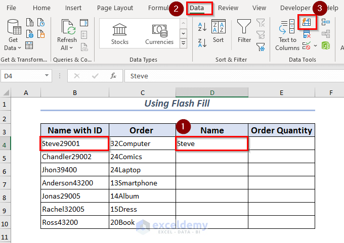
- The keyboard shortcut to use Flash Fill is Ctrl + E.
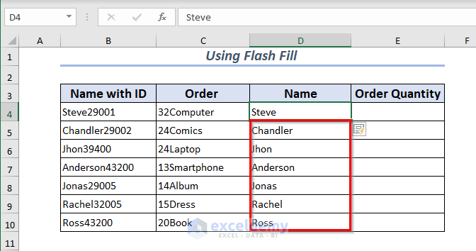
- This fills in the column based on the pattern.
- Repeat the process to extract the order number from column C into column E. You need to manually input the digits in E4 and use Flash Fill.
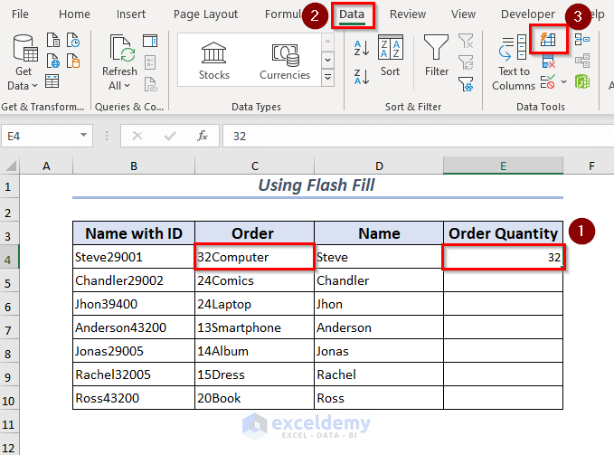
- After Flash Fill, the right characters of the rest of the cells will be removed.
Method 5 – Remove Characters From Either Side at Once
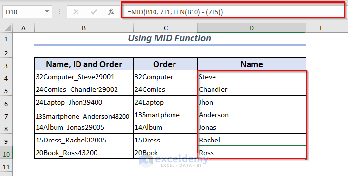
We’ll modify the dataset to include all information in a single cell, then extract pieces.
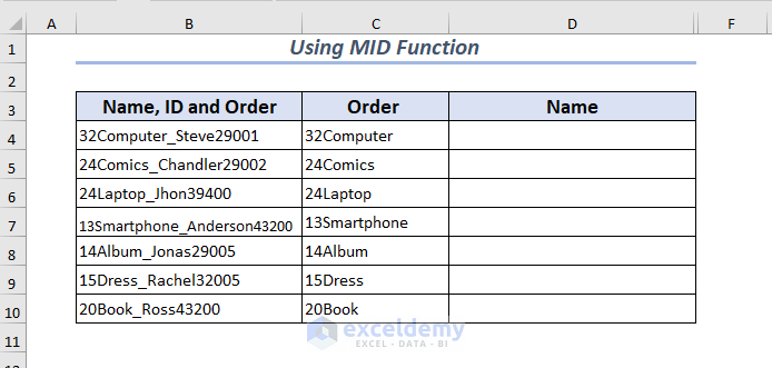
- Select a cell where you want to keep your new value after removing the character from both left and right. We chose cell D4.
- Use the following formula to extract the name from cell B4:
=MID(B4, 11+1, LEN(B4) - (10+6))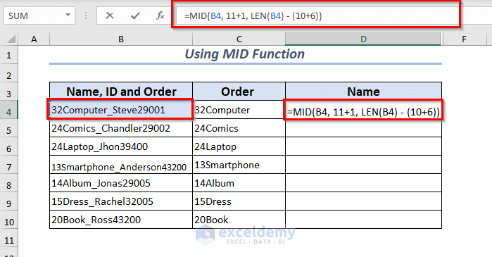
- To apply the formula, press Enter.
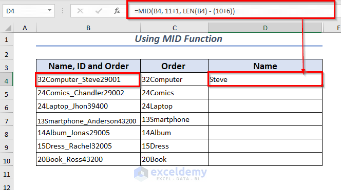
- Modify the function for the other cells depending on where the name starts in a particular cell.
Practice Section
We have attached two extra sheets to practice these methods.
Download the Practice Workbook
Excel Remove Characters from Right: Knowledge Hub
- Remove Last Character in Excel
- Remove Last Digit in Excel
- Remove the Last 3 Characters in Excel
- Remove Last Character from String Using VBA in Excel
<< Go Back To Excel Remove Characters | Data Cleaning in Excel | Learn Excel
Get FREE Advanced Excel Exercises with Solutions!

