How to Round to the Nearest 5 or 9 in Excel (8 Methods)

Dataset Overview

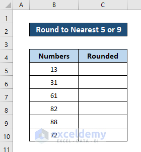
The following dataset will be used to demonstrate all of the methods.

Method 1 – Combination of ROUND, CHOOSE and MOD Functions

To round a number, we use the ROUND function for a specified number of digits. It needs two arguments, a number it is rounding and the number it is rounding to.

The CHOOSE function takes an index number and several numbers as arguments and chooses a specific action according to the index number.

The MOD function takes a number and a divisor to return the remainder.

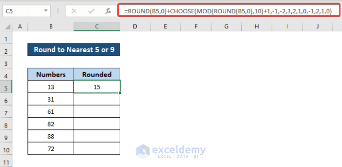
Select cell C5.
Enter the following formula in the cell:

=ROUND(B5,0)+CHOOSE(MOD(ROUND(B5,0),10)+1,-1,-2,3,2,1,0,-1,2,1,0)

Press Enter. This will round the value in cell B5 to the nearest 5 or 9.

excel round to nearest 5 or 9

Select the cell again and drag the fill handle down to apply the formula to the rest of the column.

excel round to nearest 5 or 9

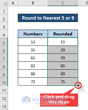
You will have the numbers rounded to the nearest 5 or 9 using the formula.

Breakdown of the Formula

The ROUND(B5,0) rounds the value of cell B5 to the nearest whole number (returns 13).

The MOD(ROUND(B5,0),10) calculates the remainder when dividing the rounded value by 10 (returns 3).

The CHOOSE(MOD(ROUND(B5,0),10)+1,-1,-2,3,2,1,0,-1,2,1,0) selects the appropriate number to add based on the remainder and original value (in this case, it’s 2).

The ROUND(B5,0)+CHOOSE(MOD(ROUND(B5,0),10)+1,-1,-2,3,2,1,0,-1,2,1,0) adds the value from the previous function to the original one.

Method 2 – Combining MROUND and MOD Functions

We use the MROUND function to return a number rounded up to desired multiple. To begin with, this function can take two arguments- the number and the multiple.

Select cell C5.
Enter the following formula:

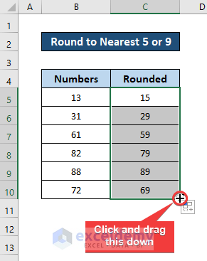
=MROUND(B5,5)-((MOD(MROUND(B5,5),10))=0)

Press Enter. This will round the value in cell B5 to the nearest 5 or 9.

excel round to nearest 5 or 9

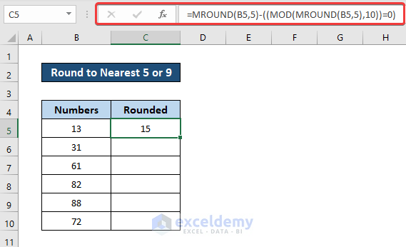
Drag the fill handle to fill out the rest of the column.

Breakdown of the Formula

MROUND(B5,5) rounds the value of cell B5 to a multiple of 5 and (returns 15).

MOD(MROUND(B5,5),10) calculates the remainder when dividing the rounded value by 10 (returns 5).

(MOD(MROUND(B5,5),10))=0 returns FALSE if the remainder is not 0.

ROUND(B5,5)-((MOD(MROUND(B5,5),10))=0) subtracts either 0 or 1, resulting in a value rounded to 5 or 9.

Method 3 – Merging IF, RIGHT and ROUND Functions

The IF function takes three arguments – a condition, a value if the condition is true and a value if that is false.

The RIGHT function accepts two arguments – a string and a number. Then it extracts those numbers from the right side of the string.

Steps:

Select cell C5.
Enter the following formula:

=IF(B5>ROUND(B5,-1),IF(RIGHT(B5)="1",ROUND(B5,-1)-1,ROUND(B5,-1)+5),IF(RIGHT(B5)="0",ROUND(B5,-1)-1,IF(RIGHT(B5)<"7",ROUND(B5,-1)-5,ROUND(B5,-1)-1)))

Press Enter.

excel round to nearest 5 or 9

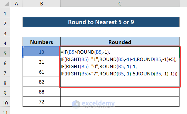
Drag the fill handle to fill the rest of the column.

excel round to nearest 5 or 9

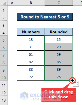
Breakdown of the Formula

The RIGHT(B5) takes the last digit of the value in cell B5.

The ROUND(B5,-1) function round the value in cell B5 to the nearest multiple of 10. In this case, it is 10.

The IF(B5>ROUND(B5,-1),…) checks whether the value is greater than the rounded number or not.

If it is, it moves on to the IF(RIGHT(B5)=”1″,ROUND(B5,-1)-1,ROUND(B5,-1)+5) section, where it checks the last digit is 1. At this point, if it is 1, then it subtracts 1 from the round value, else it adds 5 to the rounded value.

IF(RIGHT(B5)=”0″,ROUND(B5,-1)-1,…) comes into play if the first IF function’s condition was false. It first checks whether the last digit is 0 or not. If it is, then 1 is subtracted from the rounded value, else it moves on to the next IF function below.

IF(RIGHT(B5)<“7”,ROUND(B5,-1)-5,ROUND(B5,-1)-1) comes into play if all of the conditions were false. This function first checks whether the last digit is less than 7. If it is, then 5 is subtracted from the rounded value, else 1 is subtracted.

All these nested IF loops combined with other functions finally give our result.

Read More: Round Down to Nearest 10 in Excel

Method 4 – Using Formula with MOD Function

This formula is concise but may have lower accuracy when dealing with a wide range of values to be rounded. It relies solely on the MOD function, which calculates the remainder of a division operation.

Select cell C5.
Enter the following formula:

=B5-MOD(B5,10)+4*(MOD(B5,10)>5)+5

Press Enter.

excel round to nearest 5 or 9

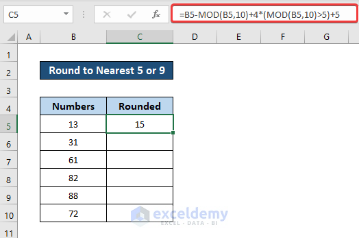
Select the cell again and drag the fill handle icon to fill up the rest of the cells.

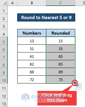
Breakdown of the Formula

MOD(B5,10) returns the remainder when dividing the value in cell B5 by 10 (in this case, it’s 3).

(MOD(B5,10)>5)evaluates to false because the remainder is smaller than 5.

And MOD(B5,10)+4*(MOD(B5,10)>5)results in 3 (the remainder).

B5-MOD(B5,10)+4*(MOD(B5,10)>5)+5 subtracts 3 from the value in cell B5.

Method 5 – Incorporating IF, RIGHT and CEILING Functions

This formula is a combination of IF, OR, RIGHT, MAX, and CEILING functions to round numbers to the nearest 5 or 9 based on specific conditions.

Select cell C5.
Enter the following formula:

=IF(OR(RIGHT(B5,1)={"0","1","2","3","4"}),MAX(CEILING(B5+1,5),0),MAX(CEILING(B5+1,10)-1,0))

Press Enter.

excel round to nearest 5 or 9

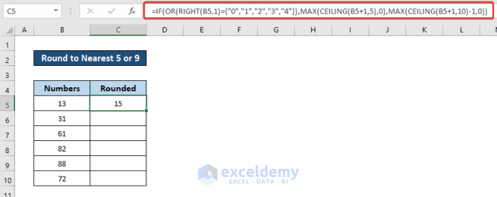
Select the cell again and drag the fill handle icon to the end of the column to fill up the rest of the cells with the formula.

excel round to nearest 5 or 9

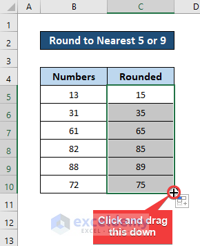
As a result, the formula will round up the values to the nearest 5 or 9 in Excel.

Breakdown of the Formula

RIGHT(B5,1) extracts the last digit from cell B5 (which is 3).

OR(RIGHT(B5,1)={“0″,”1″,”2″,”3″,”4”}) evaluates to TRUE because the last digit matches the specified list.

CEILING(B5+1,5) returns the value 15.

MAX(CEILING(B5+1,5),0) results in 15 if the final condition of the IF function is true.

MAX(CEILING(B5+1,10)-1,0) results in 19 (if the final condition of the IF function is false).

IF(OR(RIGHT(B5,1)={“0″,”1″,”2″,”3″,”4”}),MAX(CEILING(B5+1,5),0),MAX(CEILING(B5+1,10)-1,0)) returns one of these values.

Method 6 – Combining IF with RIGHT Function in Excel

Select cell C5.
Enter the following formula:

=B5-RIGHT(B5,1)*1+IF(RIGHT(B5,1)*1<6,5,9)

Press Enter.

excel round to nearest 5 or 9

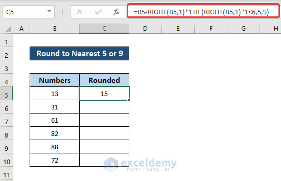
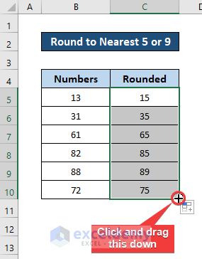
Select the cell again. Drag the fill handle icon to fill up the rest of the cells of the column with the formula.

Breakdown of the Formula

RIGHT(B5,1) extracts the rightmost digit from cell B5 (which is 3).

RIGHT(B5,1)*1 also returns the value 3.

IF(RIGHT(B5,1)*1<6,5,9) evaluates to TRUE.

B5-RIGHT(B5,1)*1+IF(RIGHT(B5,1)*1<6,5,9) results in the value 15 after all the algebraic calculations.

Method 7 – Using a Combination of CEILING and MOD Functions

Select cell C5.
Enter the following formula:

=CEILING(B5+(MOD(B5,2)=0),5)-(MOD(CEILING(B5+(MOD(B5,2)=0),5),2)=0)

Press Enter.

excel round to nearest 5 or 9

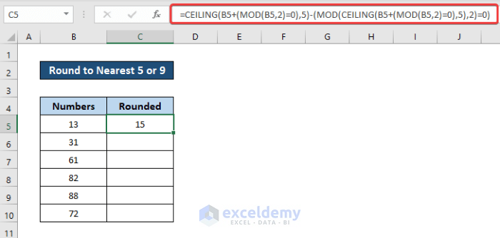
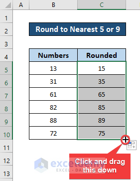
Select the cell again. Drag the fill handle icon to fill up the rest of the cells with the formula.

excel round to nearest 5 or 9

Breakdown of the Formula

MOD(B5,2) returns the remainder when dividing the value of cell B5 by 2 (in this case, it’s 1).

MOD(B5,2)=0 evaluates to FALSE because the remainder is not 0.

CEILING(B5+(MOD(B5,2)=0),5) rounds the original value up to a multiple of 5 (returns 15).

MOD(CEILING(B5+(MOD(B5,2)=0),5),2) calculates the remainder of the rounded value divided by 2.

MOD(CEILING(B5+(MOD(B5,2)=0),5),2)=0 evaluates to TRUE.

The result of the algebraic operations in CEILING(B5+(MOD(B5,2)=0),5)-(MOD(CEILING(B5+(MOD(B5,2)=0),5),2)=0) returns the value that rounds to the nearest 5 or 9.

Method 8 – Embedding VBA Code

Enable the Developer Tab:
- If you don’t see the Developer tab in your Excel ribbon, you’ll need to enable it. Here’s how:
  - Go to the File tab.
  - Click on Options.
  - In the Excel Options dialog, select Customize Ribbon on the left.
  - Check the box next to Developer under the Main Tabs section.
  - Click OK to save the changes.

Access the VBA Editor:
- Click on the Developer tab in the ribbon.
- Select Visual Basic from the Code group. This opens the VBA editor.

excel round to nearest 5 or 9

Create a New Module:
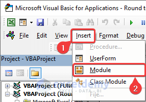
- In the VBA editor, click on Insert and choose Module from the drop-down menu.
- A new module will appear in the project explorer.

Insert the Custom Function:
- In the newly created module, insert the following VBA code:

Function Round59(number As Double)
    Dim N As Single, M As Single
    N = Int(number / 10) * 10
    M = number - N
    If M >= 2 And M < 7 Then
        M = 5
    Else
        If M >= 7 Then
            M = 9
        Else
            M = 9
            N = N - 10
        End If
    End If
    Round59 = N + M
End Function

Save and Close the VBA Editor:
- Save your workbook to retain the custom function.
- Close the VBA editor.

Apply the Custom Function:
- Go back to your spreadsheet.
- Select cell C5 (or any other cell where you want to insert the custom function).
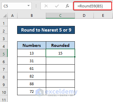
- Enter the following formula:

=Round59(B5)

Press Enter.

excel round to nearest 5 or 9

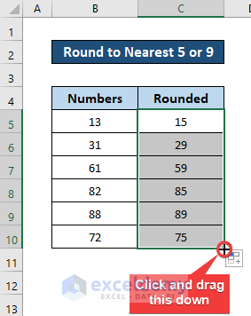
Fill Down:
- Select the cell with the formula.
- Click and drag the fill handle (the small square at the bottom-right corner of the cell) down to fill the rest of the column with the formula.