Here’s an overview of the ROUNDUP function and its most common uses.
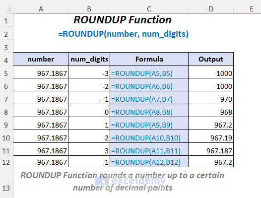
ROUNDUP Function: Syntax & Arguments
⦿ Function Objective
The ROUNDUP function rounds a number away from zero.
⦿ Syntax
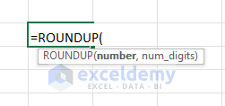
ROUNDUP(number, num_digits)
⦿ Arguments
| Argument | Required/Optional | Explanation |
|---|---|---|
| number | Required | The number to round up. |
| num_digits | Required | The place at which the number should be rounded. |
⦿ Return Value
The ROUNDUP function returns a rounded number.
⦿ Version
The ROUNDUP function has been introduced in Excel 2003 version and is available for all subsequent versions.
How to Use the ROUNDUP Function in Excel: 6 Examples
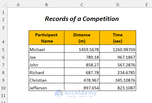
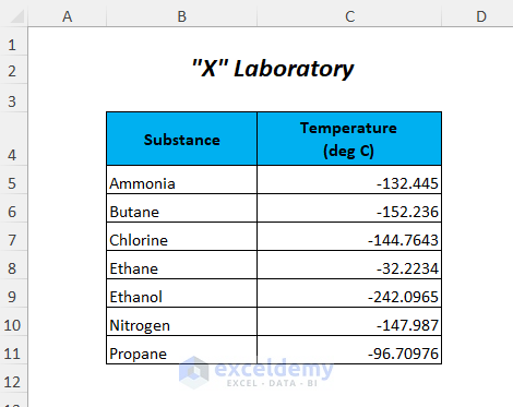
We’ll use the following two tables for demonstrating the applications of the ROUNDUP function in Excel.
Example 1 – Rounding a Number Up to The Nearest Whole Number
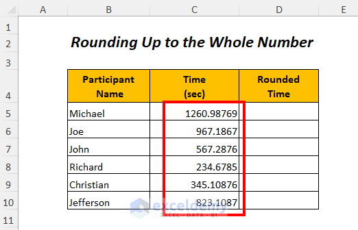
We will round up the times of the following table to the nearest whole number by using the ROUNDUP function.
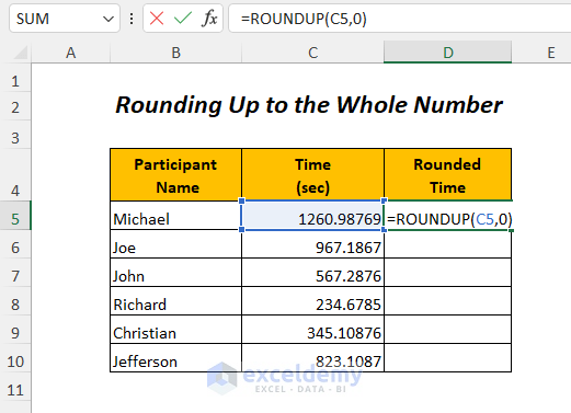
- Insert the following formula in the first output cell (D5):
=ROUNDUP(C5,0)Here, C5 is the time which we want to round up and 0 is the number digit that will round up the value to the nearest whole number.
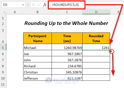
- Hit Enter and drag down the Fill Handle to fill the column.
Result:
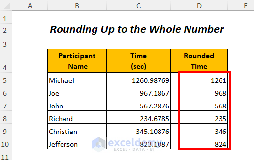
You can also get the result by inserting a direct input instead of reference:
=ROUNDUP(1260.98769,0)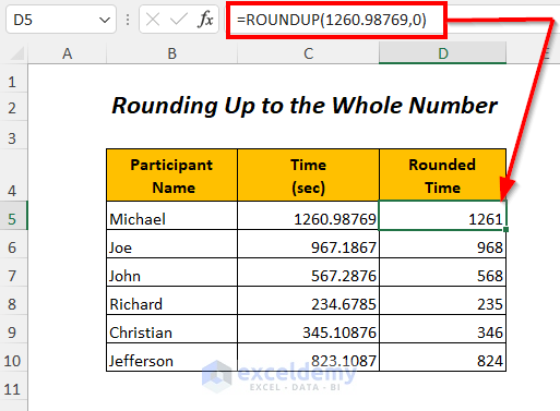
Example 2 – Rounding a Number Up with a Positive Number Digit
You can round up the values for any positive number digits to the right of the decimal point by using the ROUNDUP function.
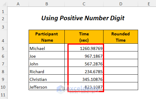
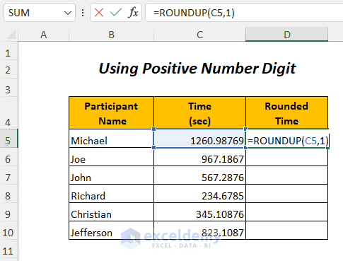
- Insert the following formula in the first output cell (D5):
=ROUNDUP(C5,1)Here, C5 is the time which we want to round up and 1 is the number digit that will round up the value to 1 decimal place.
- Hit Enter and drag down the Fill Handle tool.
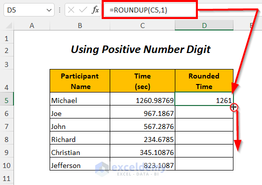
Result:
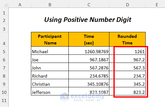
You can round up to two places right of the decimal point by using the following formula:
=ROUNDUP(C5,2)Here, C5 is the time which we want to round up and 2 is the number digit that will round up the value to 2 decimal places.

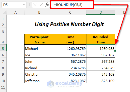
For rounding up the times to three places right of the decimal point, you can use the following formula:
=ROUNDUP(C5,3)C5 is the time which we want to round up and 3 is the number digit that will round up the value to 3 decimal places.
Example 3 – Rounding a Number Up with a Negative Number Digit
We will round up the values for any negative number digits to the left of the decimal point by using the ROUNDUP function.
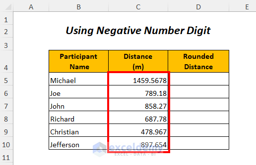
- Insert the following formula in the first output cell (D5):
=ROUNDUP(C5,-1)Here, C5 is the distance which we want to round up and –1 is the number digit. This negative number will round up the value to the nearest 10.
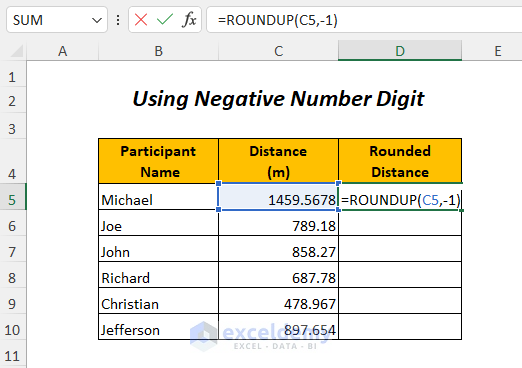
- Press Enter and drag down the Fill Handle.
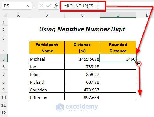
Result:
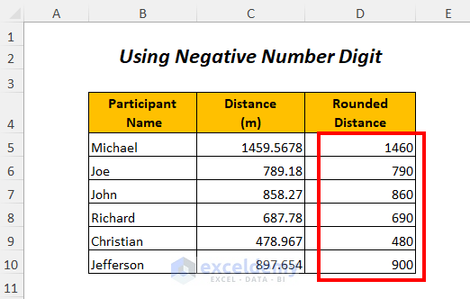
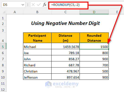
You can round up the distances to two places left of the decimal point by using the following formula:
=ROUNDUP(C5,-2)Here, C5 is the distance which we want to round up and –2 is the number digit that will round up the value to the nearest 100.
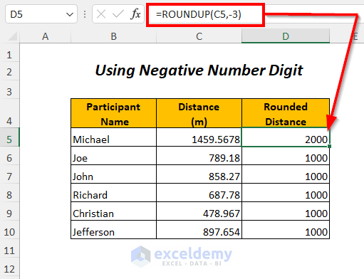
For rounding up the distances to three places left of the decimal point, you can use the following formula:
=ROUNDUP(C5,-3)C5 is the distance which we want to round up and –3 is the number digit that will round up the value to the nearest 1000.
Example 4 – Using The ROUNDUP Function in a Formula
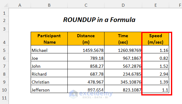
We will determine the speed of the participants by dividing the distances by times and round up the values to the two decimal places.
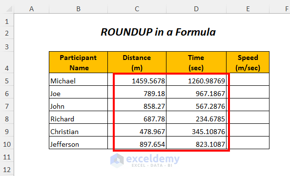
- Insert the following formula in the first output cell (E5):
=ROUNDUP((C5/D5),2)C5 is the distance and D5 is the time
- (C5/D5)→Divides the distance by the time.
Output→1.15748
- ROUNDUP((C5/D5),2) becomes
ROUNDUP(1.15748,2)→Rounds up the value to two decimal places by using the number digit 2.
Output→1.16
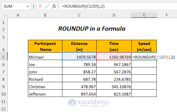
- Hit Enter and use the Fill Handle to AutoFill.
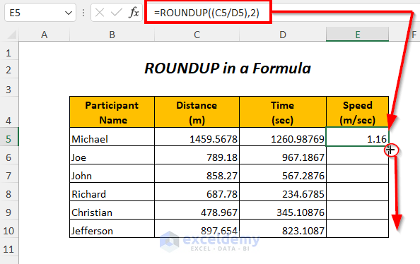
Result:
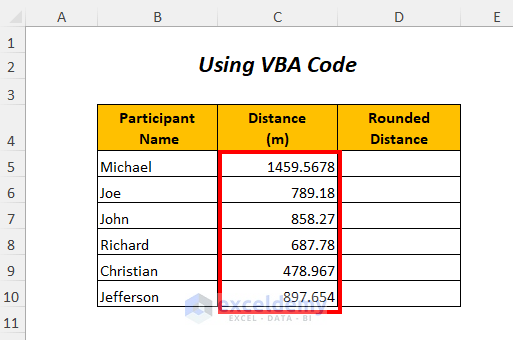
Example 5 – Using The ROUNDUP Function in VBA Code
You can use the ROUNDUP function in the VBA code also.
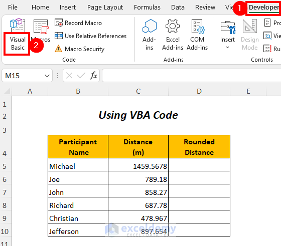
- Go to the Developer tab and select Visual Basic.
- The Visual Basic Editor will open up.
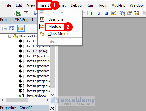
- Go to the Insert tab and select the Module option.
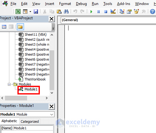
- A Module will be created.
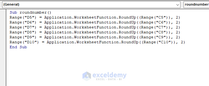
- Insert the following code:
Sub roundnumber()

    Range("D5") = Application.WorksheetFunction.RoundUp((Range("C5")), 2)
    Range("D6") = Application.WorksheetFunction.RoundUp((Range("C6")), 2)
    Range("D7") = Application.WorksheetFunction.RoundUp((Range("C7")), 2)
    Range("D8") = Application.WorksheetFunction.RoundUp((Range("C8")), 2)
    Range("D9") = Application.WorksheetFunction.RoundUp((Range("C9")), 2)
    Range("D10") = Application.WorksheetFunction.RoundUp((Range("C10")), 2)

End Sub
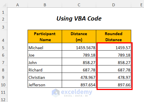
ROUNDUP will round up the values of the cells C5 to C10 of Column C to 2 decimal places and we will get the outputs in corresponding cells of Column D.
- Press F5.
Result:
Example 6 – Using the ROUNDUP Function for Negative Values
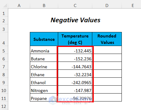
For the negative temperature of the substances, you can also round them up by using the ROUNDUP function.
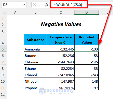
- We will try to get the nearest negative integers by using the following formula
=ROUNDUP(C5,0)C5 is the negative temperature that we want to round up and 0 is the number digit that will round up the value to the nearest whole number.
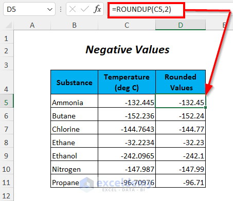
- You can round up the negative temperatures to two places right of the decimal point by using the following formula.
=ROUNDUP(C5,2)C5 is the negative temperature that we want to round up and 2 is the number digit that will round up the value to 2 decimal places.
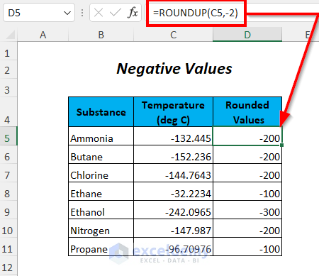
- For rounding up the negative temperatures to two places left of the decimal point, you can use the following formula.
=ROUNDUP(C5,-2)C5 is the negative temperature that we want to round up and –2 is the number digit that will round up the value to the nearest 100.
Practice Section
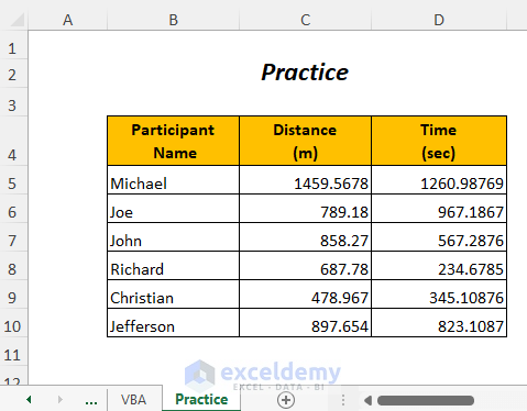
We have provided a Practice section like below in a sheet named Practice.
Download the Practice Workbook
<< Go Back to Excel Functions | Learn Excel
Get FREE Advanced Excel Exercises with Solutions!

