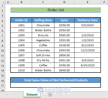
Suppose we have a dataset of some delivered products, with details for Order ID, Selling Item, Sales, and Delivery Date.

Using the SUMIF function with the ISBLANK function, let’s calculate the Total Sales value for the products that were not delivered, represented in our dataset by blank cells in the Delivery Date column.
We used the Microsoft Excel 365 version in this tutorial.
Method 1 – Combining ISBLANK with SUM and IF Functions to Get Sum of Blank Cells
Steps:
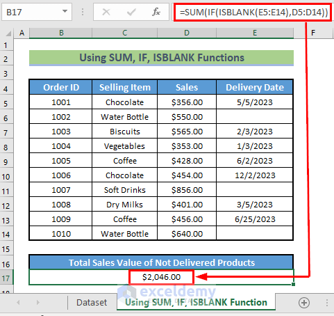
- In cell B17, enter the following formula, and press ENTER:
=SUM(IF(ISBLANK(E5:E14), D5:D14))

Formula Breakdown:
- ISBLANK(E5:E14) → The ISBLANK function will search for the empty cells in the Delivery Date column.
- E5:E14 → is the range of the cells where the ISBLANK function will search.
- Output → the range of cells where TRUE and FALSE are stored.
- E5:E14 → is the range of the cells where the ISBLANK function will search.
- IF(ISBLANK(E5:E14), D5:D14) → returns FALSE if the cell contains FALSE and returns the value of the respective Sales column if the cell contains TRUE.
- Output → the range of cells containing Sales values and FALSE.
- SUM(IF(ISBLANK(E5:E14), D5:D14)) → becomes
- SUM(D6, D11, D14) → which adds the selected cells together.
- Output → $2046.00.
- SUM(D6, D11, D14) → which adds the selected cells together.
Read More: How to Use ISBLANK Function to Check If Cell Is Blank in Excel
Method 2 – Using SUMIF Function with Empty String Criteria to Add Values for Blank Cells in Excel
We can also use just the SUMIF function to calculate the Total Sales of the blank cells in our dataset.
Steps:
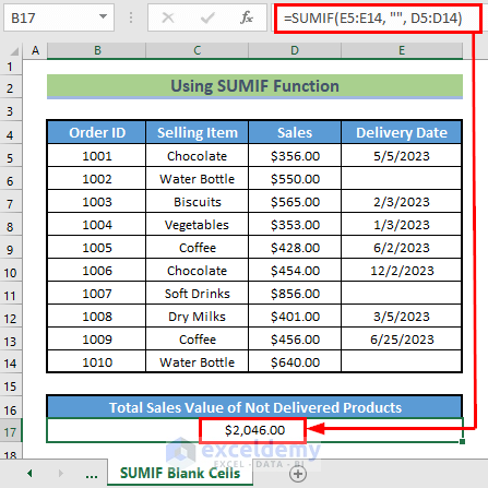
- In cell B17, enter the following formula, and press ENTER:
=SUMIF(E5:E14, "", D5:D14)
Formula Breakdown:
- SUMIF(E5:E14, “”, D5:D14) → The SUMIF function will search cells in the Delivery Date column for blank cells, and sum the corresponding Sales values.
- E5:E14 → is the range where the SUMIF function will search for blank cells.
- “” → is the criteria for finding blank cells in the range. It is used to search for finding zero-character-length cells.
- D5:D14 → is the range of cells to sum.
- Output → $2046.00.
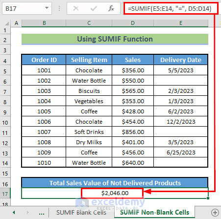
Alternatively, we can substitute “” with = in the formula above as follows:
=SUMIF(E5:E14, "=", D5:D14)
Formula Breakdown
- SUMIF(E5:E14, “=”, D5:D14) → The SUMIF function will search cells in the Delivery Date column and specify non-blank cells, to sum up, the corresponding Sales value.
- E5:E14 → is the range where the SUMIF function will search for non-blank cells.
- “=” → is the criteria for finding non-blank cells in the range.
- D5:D14 → is the range of cells to add up.
- Output → $2046.00.
Read More: How to Use ISBLANK Function for Conditional Formatting in Excel
Things to Remember
- The LEN and TRIM functions can be used to ‘blank’ cells with unseen characters like spaces. But since LEN and TRIM are text functions, they can’t be applied to the above dataset of numeric values.
- However we can use an ISBLANK function to check for spaces and hidden characters. The function checks whether the cell is empty or not, and returns TRUE or FALSE accordingly. A FALSE result indicates that the cell is not actually blank.
Download Practice Workbook
Related Articles
- How to Use ISBLANK Function in Excel for Multiple Cells
- How to Use Excel ISBLANK to Identify Blanks in Range
- Excel ISBLANK vs IsEmpty
<< Go Back to Excel ISBLANK Function | Excel Functions | Learn Excel
Get FREE Advanced Excel Exercises with Solutions!

