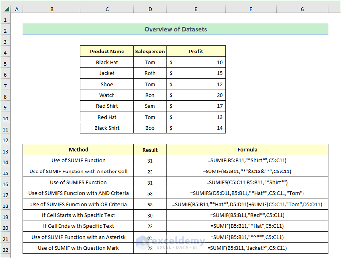
This tutorial uses a dataset for Product Name, Salesperson, and Profit, as shown below:
Download Practice Workbook
You can download the free Excel template here.
9 Easy Ways to Use SUMIF with Text in Excel
Method 1 – SUMIF with a Specific Text
This tutorial focuses on the following dataset.
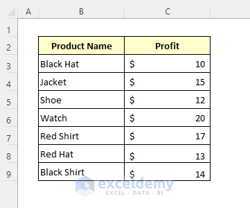
Steps:
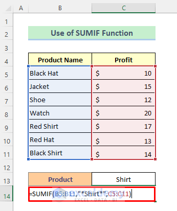
- Select Cell C14.
- Type the formula given below:
=SUMIF(B5:B11,"*Shirt*",C5:C11)- Hit the Enter key.
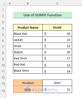
- Notice the sum of the “Shirt” items.
Read More: How to Sum Names in Excel (4 Suitable Ways)
Method 2 – SUMIF with Cell Reference of a Text in Excel
Steps:
- In cell C14, type the formula given below:
=SUMIF(B5:B11,"*"&C13&"*",C5:C11)- Hit the Enter key for the result.
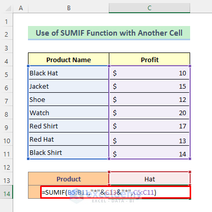
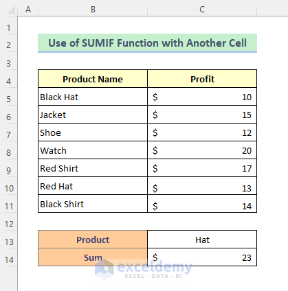
Here is the result:
Read More: How to Assign Value to Text and Sum in Excel (2 Easy Methods)
Method 3 – Apply Excel SUMIFS Function with Specific Text
Steps:
- Type the formula in Cell C14:
=SUMIFS(C5:C11,B5:B11,"*Shirt*")- Hit the Enter key.
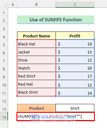
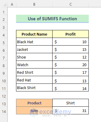
This is the result.
Read More: Sum If a Cell Contains Text in Excel (6 Suitable Formulas)
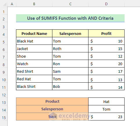
Method 4 – Use of SUMIFS with Multiple AND Criteria in Excel
This method adds a new column: “Salesperson.”
Steps:
- Type this formula in cell D15:
=SUMIFS(D5:D11,B5:B11,"*Hat*",C5:C11,"Tom")- Press the Enter key.

Notice the result with the calculation AND criteria.
Read More: How to Sum Cells with Text and Numbers in Excel
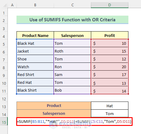
Method 5 – Use of SUMIF with Multiple OR Criteria in Excel
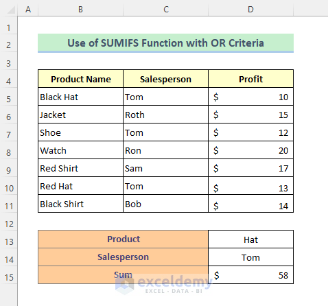
This method uses multiple criteria, specifically Hat OR Tom.
Steps:
- Type the formula in Cell D15:
=SUMIF(B5:B11,"*Hat*",D5:D11)+SUMIF(C5:C11,"Tom",D5:D11)- Hit the Enter key.
Here is the result:
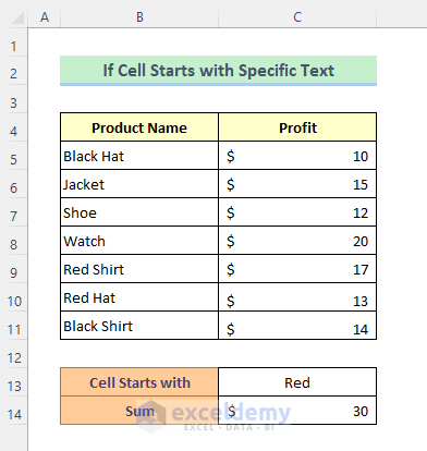
Method 6 – Use of SUMIF When Cells Start with Specific Text in Excel
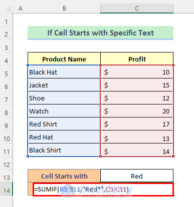
Use a Wildcard (*) to select cells starting with specific text.
Steps:
- After selecting cell C14, type the formula as given below:
=SUMIF(B5:B11,"Red*",C5:C11)- Press the Enter key.
Here is the result:
Method 7: SUMIF When Cells End with Specific Text in Excel
Use a Wildcard (*) to select cells starting with specific text.
Steps:
- Put the following in cell C14:
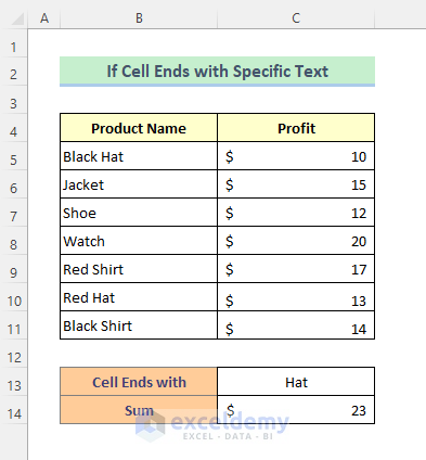
=SUMIF(B5:B11,"*Hat",C5:C11)- Hit Enter.
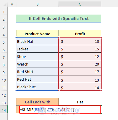
Here is the result:
Method 8 – Excel SUMIF with Text and Asterisk
Asterisk (*) represents any number of characters. For example, “Sh*” returns Shirt or Short. Tilde(~) is used to indicate the asterisk and question mark characters as they are, as * or ?, instead of a wildcard character in the formula. For example, “Sh~*” returns Sh* but not Shirt or Short. “*~**” in our formula means the SUMIF function will find the Asterisk(*) in any position of a cell.
Steps:
- Type the formula below in cell C13:
=SUMIF(B5:B11,"*~**",C5:C11)- Press the Enter key.
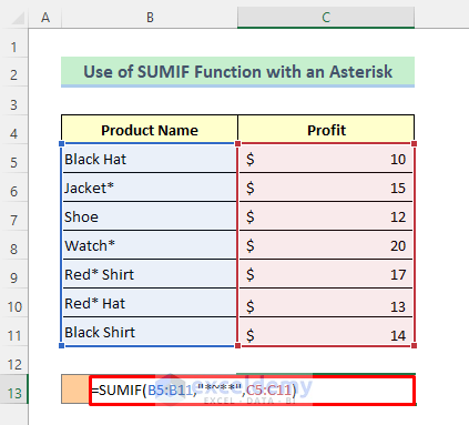
Notice the result for the cells that an asterisk.
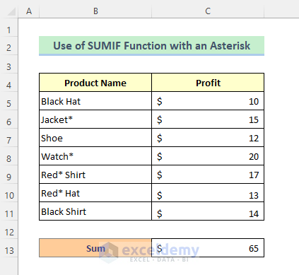
Note: To sum the profit of the cells where Asterisk is at the end of the text only, then just use “*~*” instead of “*~**”.
Read More: How to Sum Text Values Like Numbers in Excel (3 Methods)
Method 9 – SUMIF with Text and Question Mark for Missing Character in a Specific Position
A Question mark(?) represents one single character.
Steps:
- Type this formula in cell C14:
=SUMIF(B5:B11,"Jacket?",C5:C11)- Hit the Enter key.
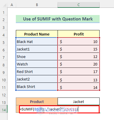
Here is the result:
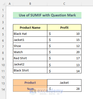
Related Articles
- How to Sum If Cell Contains Text in Another Cell in Excel
- Sum Only Numbers and Ignore Text in Same Cell in Excel


