Here’s an overview of applying the SUMIFS function in Excel.

Introduction to the SUMIFS Function

- Function Objective:
Add the cells given by specified conditions or criteria.
- Syntax:
=SUMIFS(sum_range, criteria_range1, criteria1, [criteria_range2], [criteria2],…)
- Arguments Explanation:
| Arguments | Required/Optional | Explanation |
|---|---|---|
| sum_range | Required | Range of cells that has to be summed under conditions or criteria. |
| criteria_range1 | Required | Range of cells where the criteria or condition will be applied. |
| criteria1 | Required | Condition for the criteria_range1. |
| [criteria_range2] | Optional | 2nd range of cells where the criteria or condition will be applied. |
| [criteria2] | Optional | Condition or criteria for the criteria_range2 |
- Return Parameter:
The sum of the cells in a numeric value that meet all the given criteria.
How to Use the SUMIFS Function in Excel – 6 Handy Examples
Example 1 – SUMIFS with a Single Condition in Excel
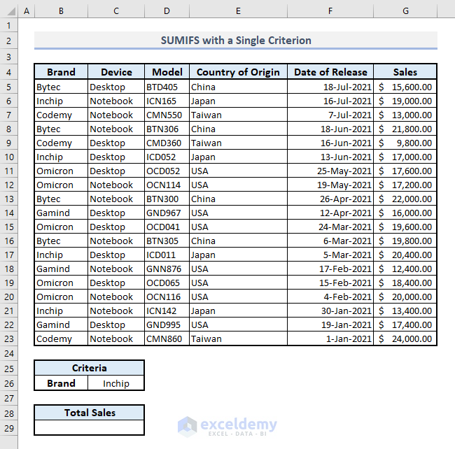
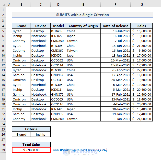
We have the sales record of computers throughout the month. We’ll sum the total sales for a single criterion, such as for devices from the Inchip brand.
Steps:
- Cell C26 contains the brand name we’re searching by.
- In the output Cell B29, insert the following:
=SUMIFS(G5:G23,B5:B23,C26)- Press Enter and you’ll get the total sales for Inchip devices from the table.
Example 2 – Using SUMIFS with Date Conditions in Excel
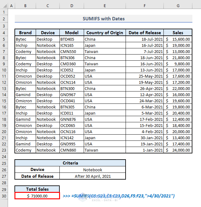
We want to know the total sales for all notebooks that were released after 30 April 2021.
Steps:
- D26 contains the value Notebook which is one condition.
- Select the output Cell C30 and insert:
=SUMIFS(G5:G23,C5:C23,D26,F5:F23,">4/30/2021")The date condition is hard-coded into the formula. However, you can enter it as text in a cell such as D27, it just needs to be in the exact format as in the formula.
- Press Enter and the function will return the total sales for all notebook devices that were released after 30 April 2021.
Read more: How to Use SUMIFS to SUM Values in Date Range in Excel
Example 3 – Using the SUMIFS Function while Excluding Blank Cells in Excel
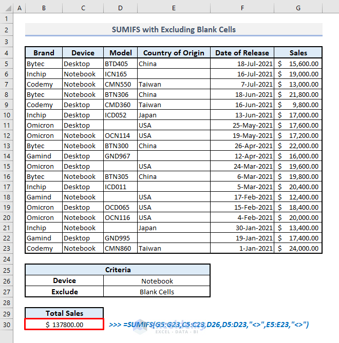
We can find the total sales value of notebook devices that have complete information in the table.
Steps:
- In the output Cell B30, apply the following formula:
=SUMIFS(G5:G23,C5:C23,D26,D5:D23,"<>",E5:E23,"<>")- Hit Enter.
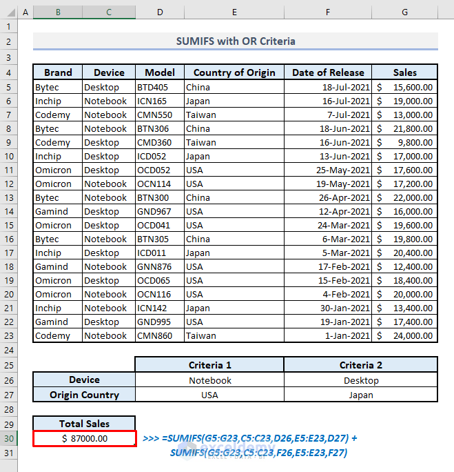
Example 4 – SUMIFS with Multiple OR Logic in Excel
We want to evaluate the sum of total sales for all notebooks that originated in the USA and all desktops that originated in Japan.
Steps:
- The conditions are in D26, D27, F26, and F27 (Notebook, USA, Desktop, Japan).
- In Cell B30, insert the following:
=SUMIFS(G5:G23,C5:C23,D26,E5:E23,D27)+SUMIFS(G5:G23,C5:C23,F26,E5:E23,F27)- Press Enter and you’ll get the desired result.
Read more: Excel SUMIFS Multiple Criteria
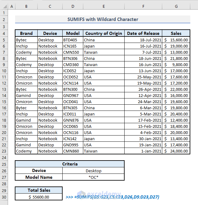
Method 5 – Inserting Wildcard Characters inside SUMIFS Function in Excel
We want to know the total sales of desktop models beginning with ‘OC’.
Steps:
- In the output Cell C30, use the following formula:
=SUMIFS(G5:G23,C5:C23,D26,D5:D23,D27)Or,
=SUMIFS(G5:G23,C5:C23,D26,D5:D23,"*OC*")- Press Enter.
Example 6 – Combining SUM and SUMIFS Functions in Excel
We want to find the total sales of all notebook devices that came from the USA and Japan.
Steps:
- The combined formula with SUM and SUMIFS functions in Cell C31 will be:
=SUM(SUMIFS(G5:G23,C5:C23,D26,E5:E23,{"USA","Japan"}))- Press Enter.
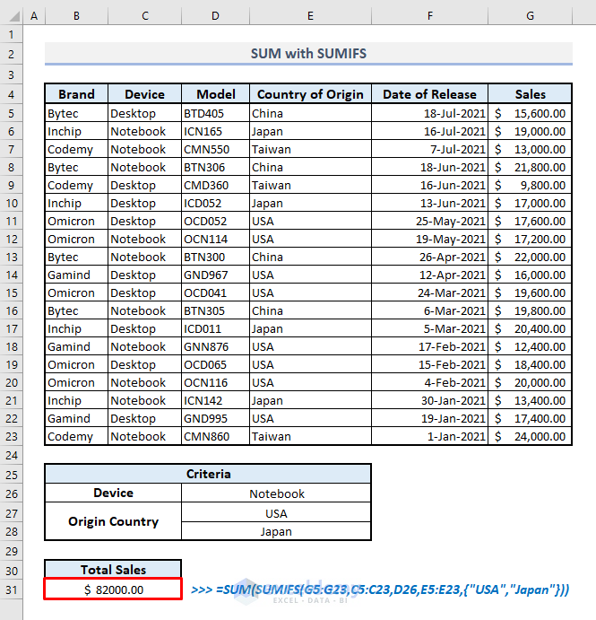
For an array input inside the SUMIFS function, the function will also return the evaluated sums in an array. The SUMIFS function will return with the total sales of the notebooks from the USA and Japan separately. The SUM function will then add the elements of the array.
SUMPRODUCT as an Alternative to the SUMIFS Function
We want to determine the total sales of the notebooks from the USA and Japan.
Steps:
- Insert the following formula in the output cell and press Enter.
=SUMPRODUCT((G5:G23)*(C5:C23=D26)*(E5:E23={"USA","Japan"}))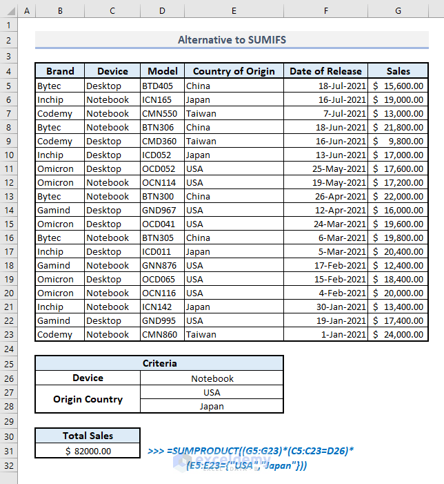
The basic difference between the uses of SUMIFS and SUMPRODUCT functions is- in the SUMIFS function you have to add and separate the range of cells and criteria with Commas (,) whereas you have to use Asterisk (*) symbol to input multiple criteria inside the SUMPRODUCT function. The SUMPRODUCT function will let you find the total sum from an array formula.
Things to Keep in Mind
The SUMIFS function will return the #SPILL error if you input an array condition inside and the function finds a merged cell in the destination.
If you input an array condition inside the SUMIFS function, it’ll return the sums for those defined conditions in an array.
If you need to evaluate the sum with a single criterion, you can use the SUMIF function instead of SUMIFS.
Unless you use the Double-Quotes(“ “) outside a text value as range criteria, the function will return zero(0) instead of showing an error.
Excel SUMIFS Function Example Download
<< Go Back to Excel Functions | Learn Excel
Get FREE Advanced Excel Exercises with Solutions!


Excellent Explanations, in a step by step manner. Most useful for me to coach my students, who can be happy by following the examples from the ages of https://www.exceldemy.com. Thanks a lot Exceldemy Team.
Hello Prabhakar Srinivasagam,
You are most welcome. Your kind words means a lot to us. We are always here to help you.
Regards
ExcelDemy