How to use the SUMPRODUCT Function Across Multiple Sheets in Excel – 2 Methods

This is an overview.

Introduction to the Excel SUMPRODUCT Function

The SUMPRODUCT function multiplies the cells of a range or array and sums them.

• Purpose 

Multiply, and then sum arrays/ranges

• Syntax 

=SUMPRODUCT (array1, [array2], …)

• Arguments

array1 – The first array or range to multiply, then add.

array2 – [optional] The second array or range to multiply, then add.

• Return value 

The result of the multiplied and summed arrays/ranges

Notes:

If a single array is supplied, the SUMPRODUCT will sum the items in the array. You can supply up to 30 arrays or ranges.

Read More: How to Use SUMPRODUCT with Criteria in Excel

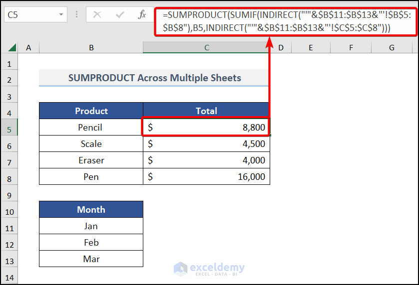
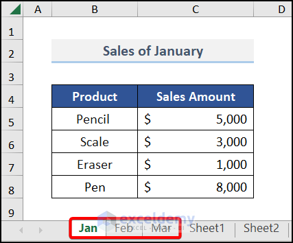
The sample dataset showcases Product and Sales Amount in the 1st 3 months of 2021 in three different sheets.

Method 1 – Applying the SUMPRODUCT, the SUMIF and the INDIRECT Functions

Introduction to the INDIRECT Function

The INDIRECT function returns the reference specified by a text string. References are immediately evaluated to display their content.

• Syntax

INDIRECT(ref_text, [a1]

• Arguments

Ref_text – A reference to a cell that contains an A1-style reference, an R1C1-style reference, a name defined as a reference, or a reference to a cell as a text string. If ref_text is not a valid cell reference, INDIRECT returns the #REF! error value.

a1 – A logical value that specifies what type of reference is contained in the cell ref_text. If a1 is TRUE or omitted, ref_text is interpreted as an A1-style reference. If a1 is FALSE, ref_text is interpreted as an R1C1-style reference.

Introduction to the SUMIF Function

The SUMIF function adds the cells specified by a given condition or criteria.

• Syntax

SUMIF(range, criteria, [sum_range])

• Arguments

range – It defines a range of cells. Cells in each range must be numbers or names, arrays, or references that contain numbers.

criteria – The criteria may be a number, expression, cell reference, text, or function. It defines which cells will be added.

Steps:

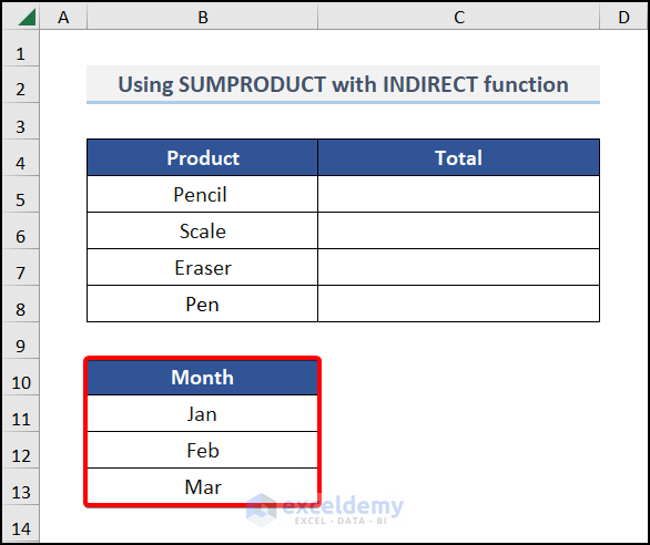
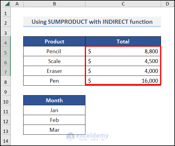
• Add the sheet names in the Month section in Sheet1.

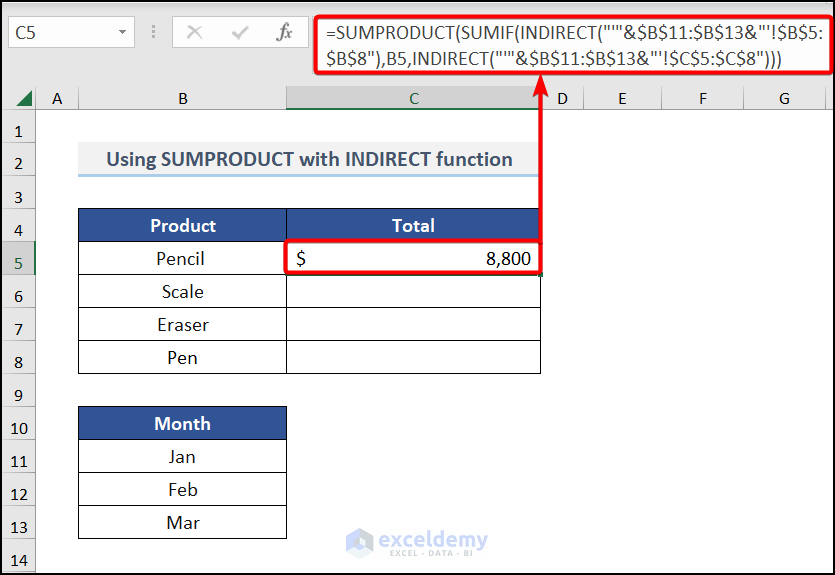
• Go to C5. and enter the formula:

• Press ENTER.

• Drag down the Fill Handle to see the result in the rest of the cells.

Read More: How to Use SUMPRODUCT Function with Multiple Columns in Excel

Method 2 – Using the SUMPRODUCT with the SUM function Across Multiple Sheets

Introduction to the SUM Function

The SUM function adds values. You can add individual values, cell references or ranges, or a mix of all three.

• Syntax

SUM(number1,[number2],…)

• Argument

number1 – The first number to add. It can be a single number, a cell reference or a cell range.

number2 – The second number to add. You can add up to 255 numbers.

Steps:

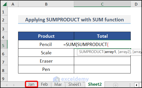
• Go to C5 in Sheet 2 and enter the SUM and SUMPRODUCT functions.
• Go to the Jan worksheet.

• Select B5:B8.

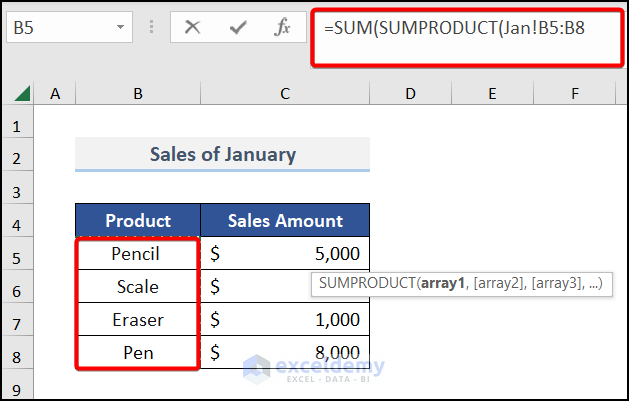
• Go to Sheet2. and inl B5, close the bracket.
• Enter a multiplication(*) sign.
• Go to the Jan worksheet .
• Select C5:C8.

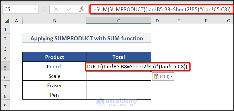
• Add Feb and Mar sheets and complete the formula. The formula becomes:

The SUM function is used to sum the SUMPRODUCT results.

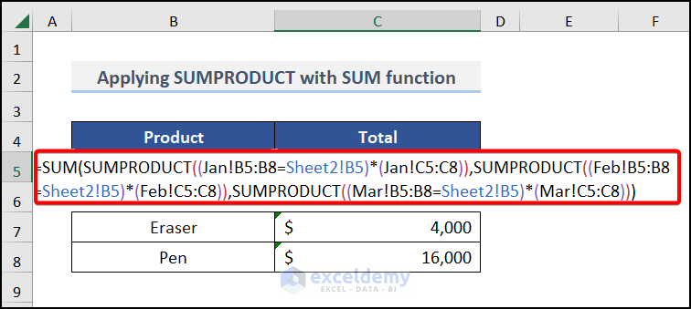
• Press ENTER.
• Drag down the Fill Handle to see the result in the rest of the cells.

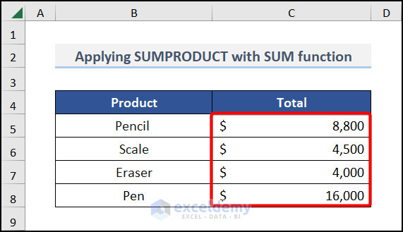
Read More: How to Use SUMPRODUCT IF in Excel

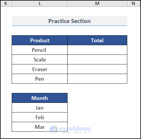
Practice Section

Practice here.

Download Practice Workbook

Download the practice workbook.

Related Articles

• SUMPRODUCT for Counting with Multiple Criteria in Excel
• [Solved] SUMPRODUCT with Multiple Criteria Not Working in Excel
• Excel SUMPRODUCT Function Based on Date Range
• How to Use SUMPRODUCT to Lookup Multiple Criteria in Excel
• Excel SUMPRODUCT with Multiple Criteria in Same Column

<< Go Back to Excel SUMPRODUCT Function | Excel Functions | Learn Excel