Method 1 – Using the Excel SWITCH Function to Switch Corresponding Cell Values
Steps:
- Enter the following formula in cell F4:
=SWITCH(C4,1,"Astron",2,"Phoenix","?")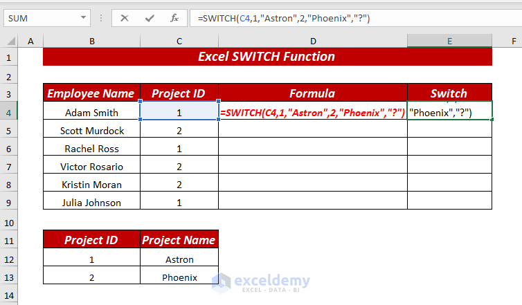
Here, in the SWITCH function, I selected the C4 cell as expression, provided 1 as value1 and Astron as a result1. Then provided 2 as value2 and Phoenix as a result2. Finally, provided ? as default.
Now, the SWITCH function will return the result by comparing the given value against the provided values.
- Press ENTER, and the SWITCH function will return the results for the provided values.
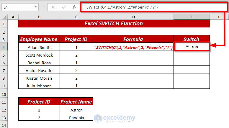
Here, you can see the Project Name Astron is assigned for the value Project Id 1.
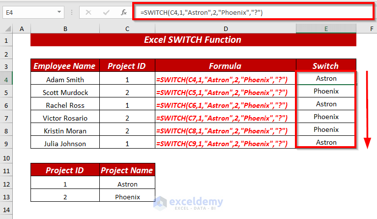
- You can follow the same process or use the Fill Handle to AutoFill the formula for the rest of the cells.
Method 2 – Using the Excel SWITCH Function with Operator
Steps:
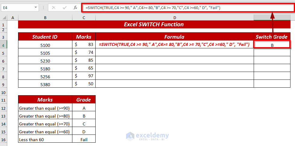
- Enter the following formula in cell E4:
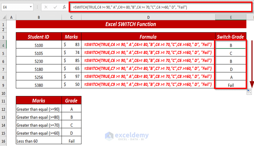
=SWITCH(TRUE,C4 >= 90," A",C4>= 80,"B",C4 >= 70,"C",C4 >=60," D", "Fail")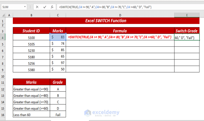
Here, in the SWITCH function, I selected the TRUE as expression, provided C4 >= 90 as value1 and A as a result1, C4>= 80 as value2, and B as result2, C4>= 70 as value3, and C as result, C4>= 60 as value4, and D as result4, finally, provided Fail as default.
Now, the SWITCH function will return the result by comparing the given value against all provided values.
- Press ENTER, and the SWITCH function will return the corresponding grades, switching the marks.
- You can follow the same process, or you can use the Fill Handle to AutoFill the formula for the rest of the cells.
Method 3 – Using the Excel SWITCH Function with the DAYS Function
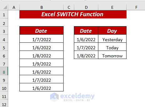
We will use the dataset below to explain the process.
Steps:
- Enter the following formula in cell C4:
=SWITCH(DAYS(TODAY(),B4), 0, "Today", 1,"Yesterday", -1,"Tomorrow","Unknown")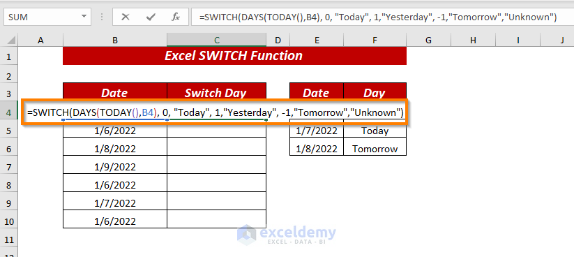
Here, in the SWITCH function, I selected the DAYS(TODAY(),B4) as expression, provided 0 as value1, and “Today” as a result1,
1 as value2, and “Yesterday” as a result2,
-1 as value3, and “Tomorrow” as a result3, finally, provided Unknown as default.
In the DAYS function, I used TODAY() as end_date and selected cell B4 as start_date.
Then, the SWITCH function will return the resultant days by comparing the given values.
- Press ENTER, and the SWITCH function will return the corresponding days, switching the dates.
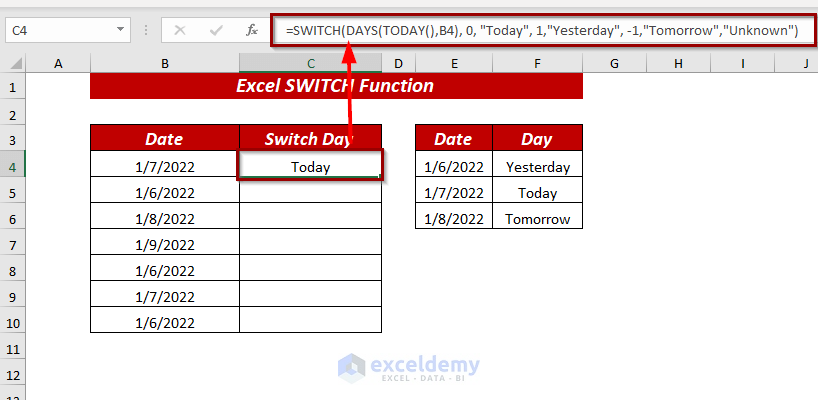
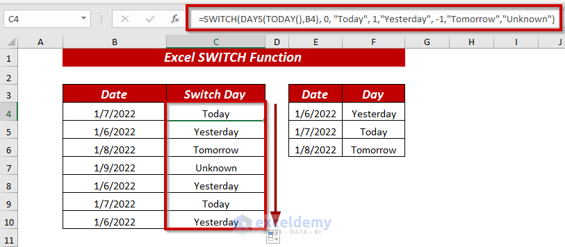
- You can follow the same process or use the Fill Handle to AutoFill the formula for the rest of the cells.
Read More: How to Use VBA Switch Function
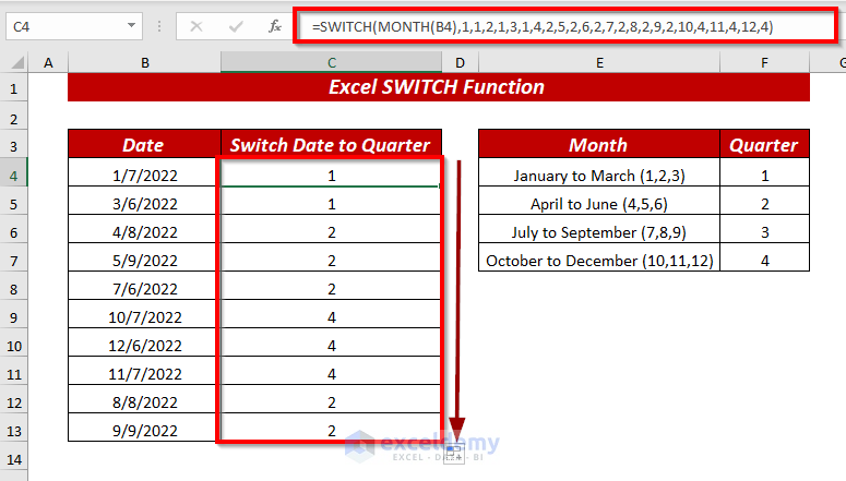
Method 4 – Using the Excel SWITCH Function with the MONTH Function
Steps:
- Enter the following formula in cell C4:
=SWITCH(MONTH(B5),1,1,2,1,3,1,4,2,5,2,6,2,7,2,8,2,9,2,10,4,11,4,12,4)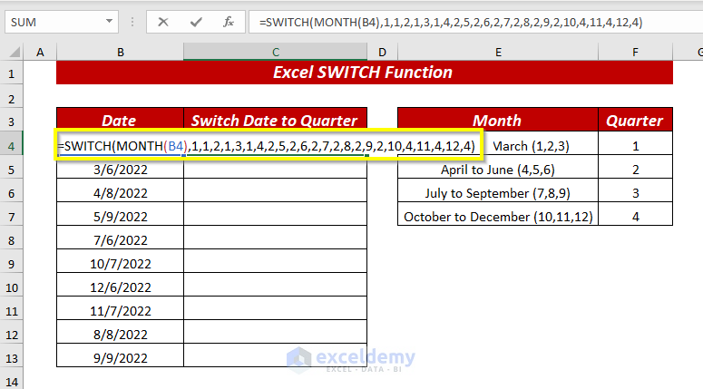
Here, in the SWITCH function, I selected the MONTH(B5) as an expression. Then, as value and result, I followed the provided chart.
Taken January to March (1,2,3) as value and provided 1 as the result
Next April to June (4,5,6) as value and provided 2 as a result. Then July to September (7,8,9) as value and provided 3 as a result, and October to December (10,11,12) as value and provided 4 as a result.
In the MONTH function, I selected the B4 cell as serial_number.
Then, the SWITCH function will return the quarter by comparing the dates.
- Press ENTER, and the SWITCH function will return the corresponding quarter, switching the dates.
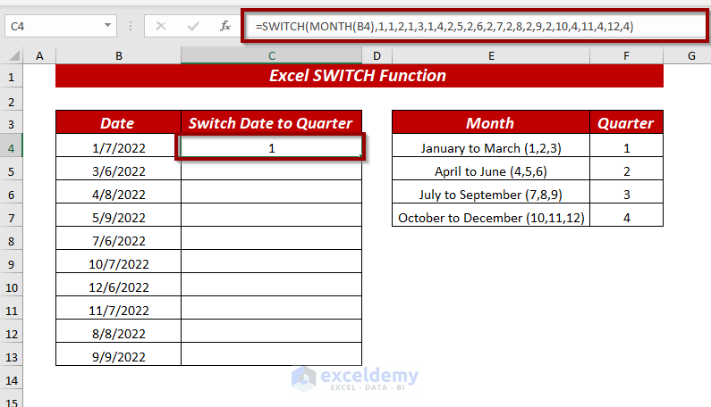
- Here, you can follow the same process, or you can use the Fill Handle to AutoFill the formula for the rest of the cells.
Method 5 – Using SWITCH & RIGHT Functions
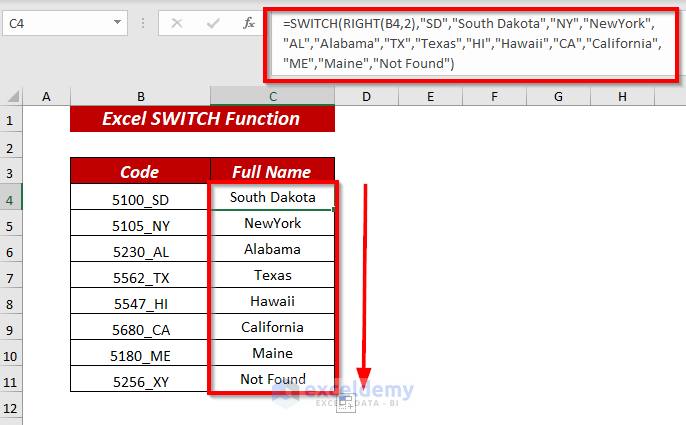
We will use the dataset below.
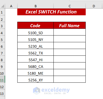
Steps:
- Enter the following formula in cell C4:
=SWITCH(RIGHT(B4,2),"SD","South Dakota","NY","NewYork","AL","Alabama","TX","Texas","HI","Hawaii","CA","California","ME","Maine","Not Found")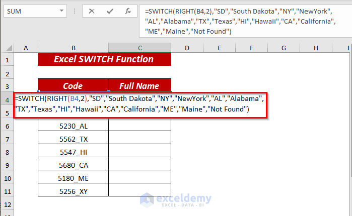
Here, in the SWITCH function, I selected the RIGHT(B4,2) as an expression.
In the RIGHT function, I selected the B4 cell as text and provided 2 as num_chars to get the last 2 characters, which are city codes.
Then, the value provided the city code and the city’s full name as a result.
After that, the SWITCH function will return the full name of the city.
- Press ENTER, and the SWITCH function will switch the city codes with the full name of the city.
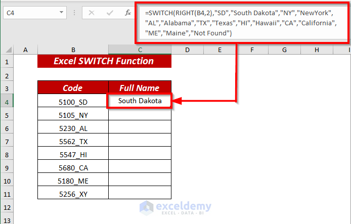
- Here, you can follow the same process, or you can use the Fill Handle to AutoFill the formula for the rest of the cells.
Comparison Between SWITCH & IFS Function
If you want, you can use the nested IF or IFS function instead of the SWITCH function.
Let me show you the comparison between the SWITCH and IFs function.
| The SWITCH Function | The IFS Function |
|---|---|
| The expression argument is used only once, | The expression argument is repeated. |
| Length is less compared to IFS | Length is larger |
| Easy to create and read | As the length is larger hard to create and read |
| Test more than one condition | Test one condition |
Things to Remember
➤ The SWITCH function can handle up to 126 pairs of values and results.
➤ You can use another function and formula as an expression.
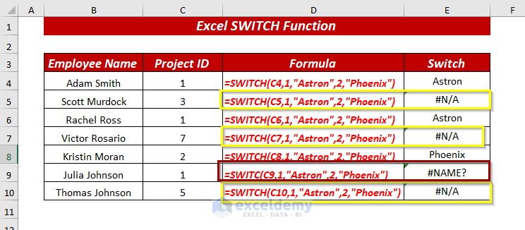
The SWITCH function shows the #N/A error if it is unable to match and there is no other argument or default condition.
➤ Whenever you get the #N/A error, then to avoid this error, you can use a string within inverted commas as the default value.
The SWITCH function will show the #NAME error if you misspell the function name.
Practice Section
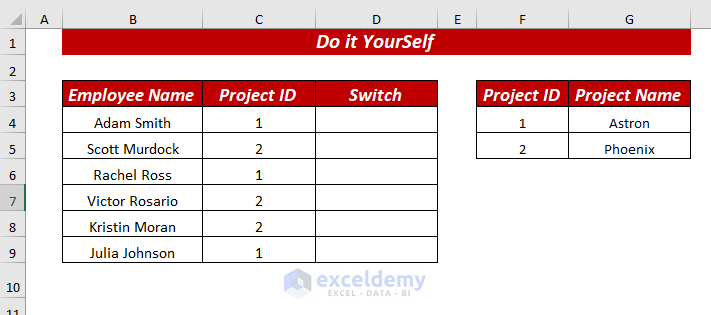
I’ve provided a practice sheet in the workbook to practice these explained examples.
Download the Practice Workbook
<< Go Back to Excel Functions | Learn Excel
Get FREE Advanced Excel Exercises with Solutions!

