The image below is a sample Weight Loss Tracker.
![]()
Download Practice Workbook
Step 1 – Calculating Weight Loss Percentage
Enter the relevant information in their corresponding cells in the form above the tracker.
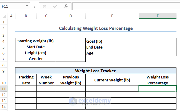
- Use the following formulas for the respective cells.
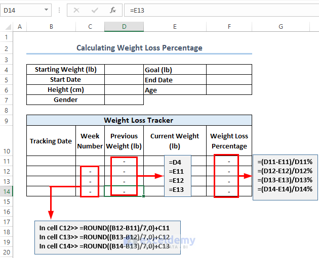
- In cell C12, enter >> =ROUND((B12-B11)/7,0)+C11
- In C13 cell, enter >> =ROUND((B13-B12)/7,0)+C12
- C14 >> =ROUND((B14-B13)/7,0)+C13
- In E11 cell, write >> =D4
- In E12, write >> =E11
- In E13 >> =E12
- In E14 >> =E13
- F11 Use >> =(D11-E11)/D11%
- Use the Fill Handle icon for other cells of the F column.
- Enter the following formula in the H5 cell to get an overall weight loss percentage.
=(D4-OFFSET(E11,COUNT(E11:E14)-1,0))/D4%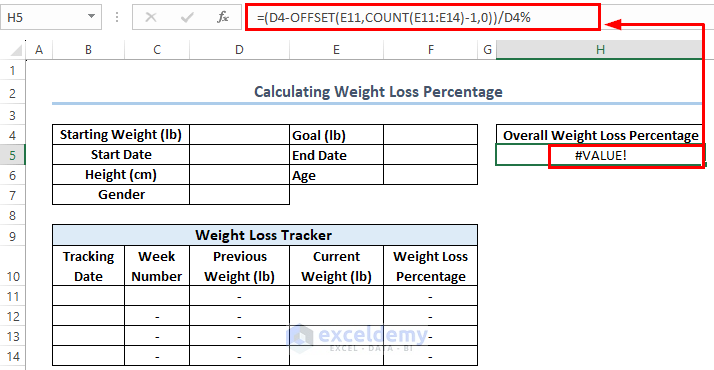
Note: To keep the % sign with the number, don’t use % symbol within formula. Change the Number format of the cell from General to Percentage.
Step 2 – Finding Weight Loss in Stones and Pounds from Kilograms
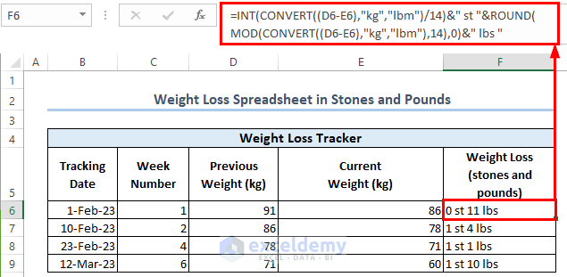
- Insert the following formula to convert kg to stones and pounds.
=INT(CONVERT((D6-E6),"kg","lbm")/14)&" st "&ROUND(MOD(CONVERT((D6-E6),"kg","lbm"),14),0)&" lbs "- Press ENTER and use the Fill Handle icon to fill the other cells of the column.
Formula Breakdown
- The CONVERT function uses these 3 arguments. The D6-E6 is the number argument, next “kg” is the from_unit argument, and lastly, “lbm” is the to_unit argument.
- Then, the INT function returns only the integer value. INT(CONVERT((D6-E6),”kg”,”lbm”)/14)—> turns 0.
- The MOD function gives the remainder of the division. The number argument is CONVERT((D6-E6)),”kg”,”lbm”, and the divisor argument is 14.
- The ROUND function rounds the above value to the nearest integer. ROUND(MOD(CONVERT((D6-E6),”kg”,”lbm”),14),0)—> gives 11.
- The “st” and “lbs” strings are joined with their corresponding values using the Ampersand (&) operator.
Step 3 – Inserting a Weight Loss Chart in Excel
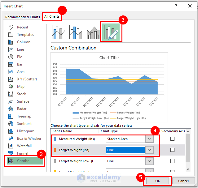
- Select the whole dataset >> go to the Insert tab > select the Recommended Charts.
- You will get the Insert Chart Go to All Charts there >> Select Combo.
- From Custom Combination, choose the Chart Type for Measured Weight as Stacked Area and set the Chart Type for Target Weight as Line >> press OK.
In the image below, I have attached the chart and some Chart Elements.
![]()
Step 4 – Calculating BMI in Excel
- The formula for BMI (Body Mass Index) is: BMI = weight(kg)/ height(meters)^2.
- Enter the following formula:
=CONVERT(C4,"lbm","kg")/(CONVERT(C5,"cm","m"))^2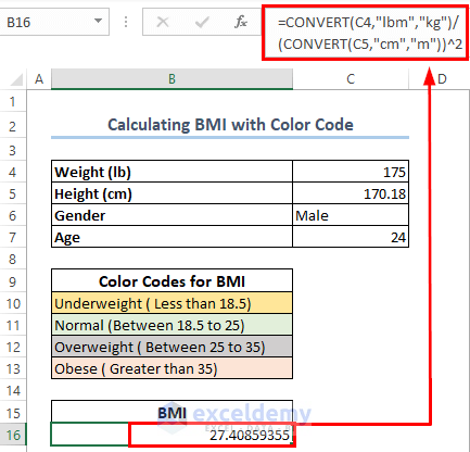
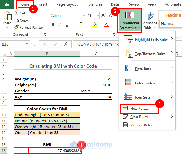
- For using color codes in BMI value, select the cell >> from the Home tab, go to Conditional Formatting >> choose New Rule.
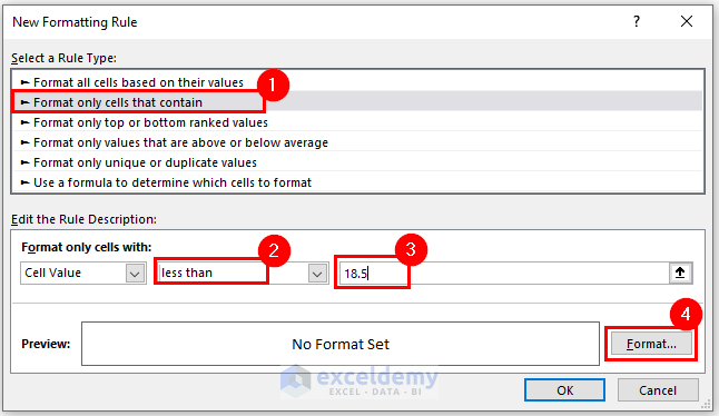
- You will get the dialog box named New Formatting Rule. Select Format only cells that contain >> go to Format only cells with: options >> choose less than >> set the value (5) >> click on Format.
- From the Format Cells dialog box >> go to Fill >> set a color >> press OK.
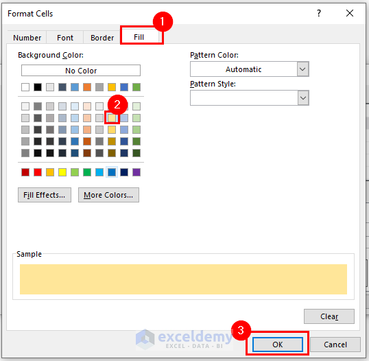
- Press OK to the New Formatting Rule dialog box.
- Set the colors using Conditional Formatting for other values.
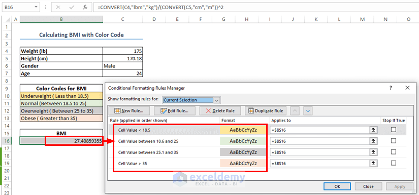
Step 5 – Combing Weight Loss Percentage, Chart and BMI to Make Tracker
Assemble the findings above for creating the weight loss tracker.
![]()
- Follow the formulas of calculating weight loss percentages.
- Add a new column named Target Weight >> link G4 cell as absolute reference.
- Use the formulas for overall weight loss percentage and BMI.
![]()
- Add the chart for tracker. We used Current Weight and Target Weight columns for the chart.
Step 6 – Checking the Output of Weight Loss Tracker in Excel
- You will need to manually fill out the form (marked red in the image below). You will get the weight loss percentage and overall weight loss percentage.
- It will also calculate the BMI and format the cell according to the color code.
- It will add the chart lines to understand the difference between current weight and target weight.
![]()
Excel Weight Loss Tracker: Knowledge Hub
<< Go Back to Tracker in Excel | Excel Templates
Get FREE Advanced Excel Exercises with Solutions!

