Overview of the TODAY Function
- Summary
The TODAY function returns the current date formatted as a date.
- Syntax
=TODAY()
The TODAY function doesn’t take any arguments in its parameter.
Note:
- The TODAY function delivers the current date and will frequently refresh each time the worksheet is updated or refreshed. Use F9 to fix the worksheet to recalculate and update the value.
- By default, this function returns the date in standard Excel date format. You can easily change the format using the Format option per your requirements.
How to Use the TODAY Function in Excel: 6 Easy Examples
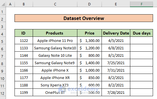
We will consider the dataset with five columns: B, C, D, E, and F for ID, Products, Price, Delivery Date, and Due Days. The dataset ranges from B4 to F12. We will use this dataset to show six easy examples of using the TODAY function in Excel.
Method 1 – Finding the Difference Between Days Using the TODAY Function
Let’s have a dataset of products with delivery dates. We will find out the due days from the delivery date to today.
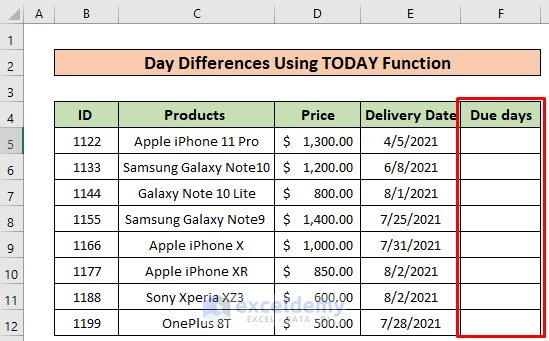
Steps:
- Enter this formula in cell F4.
=TODAY()-E4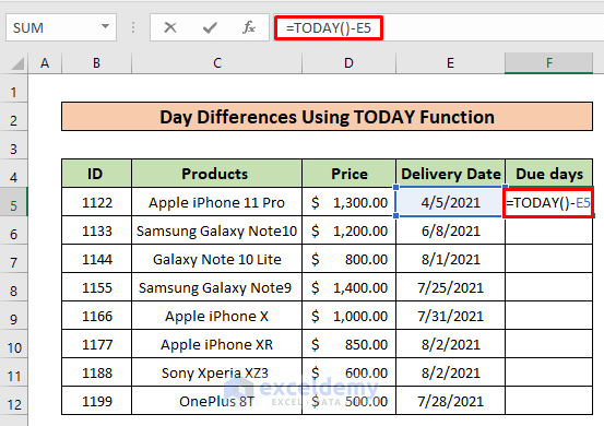
- Use the Fill handle down to F11.
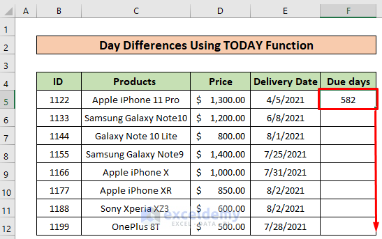
- You will see the final outcome.
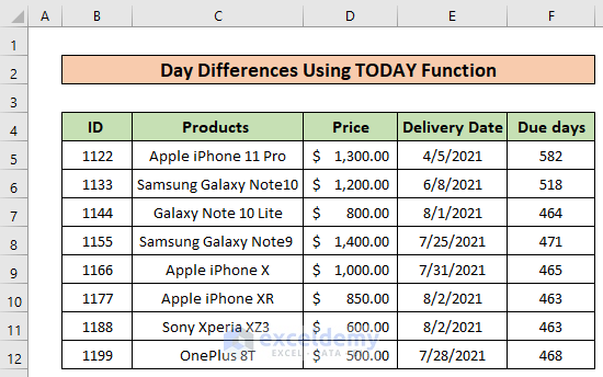
Note:
- Make sure the Due days column is in general format.
Method 2 – Find Months Since or Before a Certain Date Using the TODAY Function
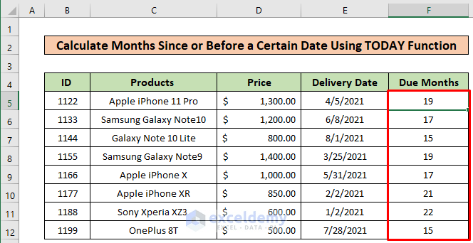
Let’s say we want to find out the Due months from the delivery dates using the same dataset above.
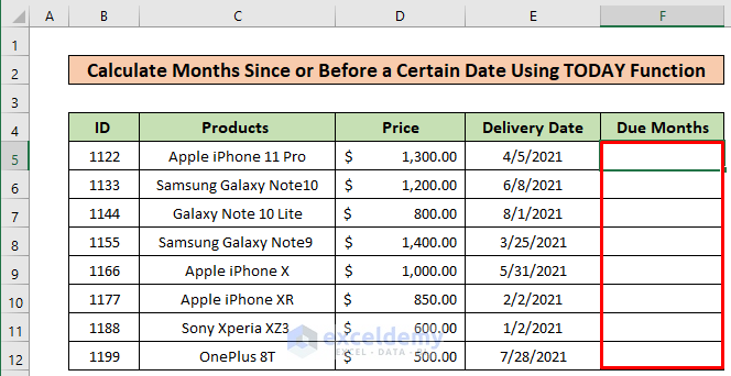
Steps:
- Enter the formula in cell F4.
=DATEDIF(E4,TODAY(),"m")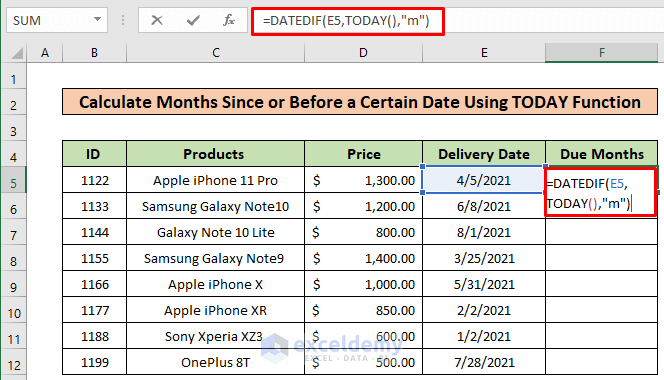
- Copy it down up to F11.
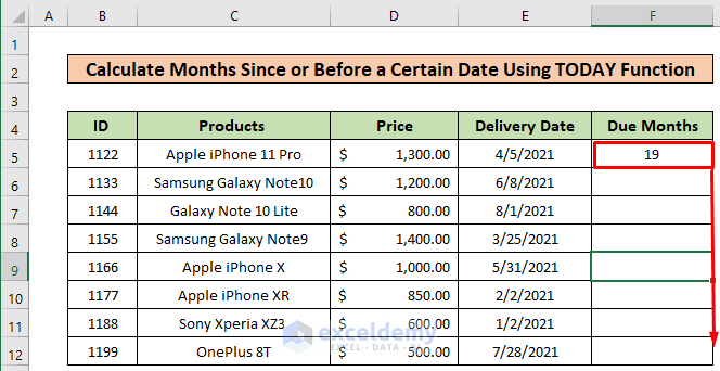
- You will get the result just like the picture given below.
How Does the Formula Work?
- As all dates start from the E4 cell, that’s why E4 is passed as the first argument.
- Our end date will be today, and we have assigned it using the TODAY function.
- As we want to return the months, “m” is used to get the number of complete months in the period.
Note:
- Make sure the Due days column is in General Format.
Method 3 – Find Years Since/Before a Certain Date Using the TODAY Function
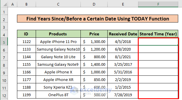
Let’s do the same thing that was done in example 2 but here instead of calculating months, we will calculate years. We will have new columns named Received Date and Stored Time (Year).
Steps:
- Enter this formula in cell F4.
=DATEDIF(E4,TODAY(),"y")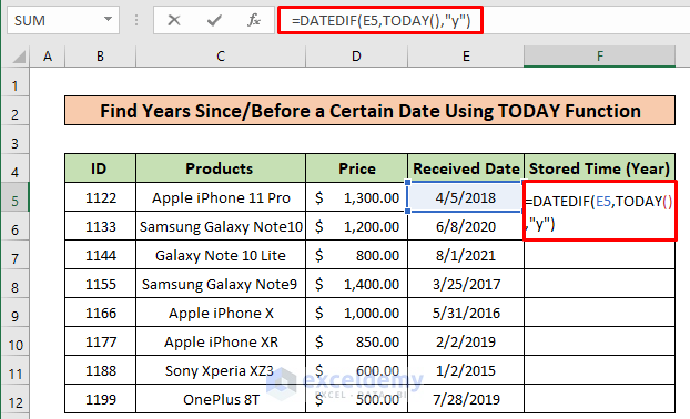
- Copy it down to F11.
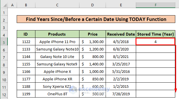
- You will get the following results.

How Does the Formula Work?
- All the arguments same as example 2 and “y” are used to get the number of years over the period.
Note:
- In cell F6, 0 is printed as the received date’s year is 2021, and the difference between Today and 8/1/2021 is 0.
Method 4 – Get an Age from a Birthdate Using the TODAY Function
Let’s have a dataset of office employees. In the dataset, we have the ID, Name, and Birthday. We want to find out the current Age of each employee.
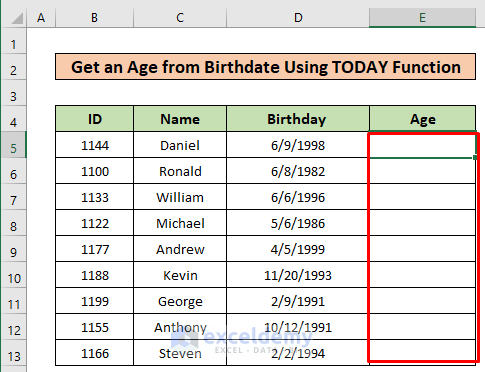
Steps:
- Enter this formula in cell E4.
=YEAR(TODAY())-YEAR(D4)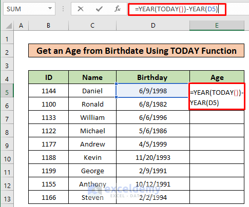
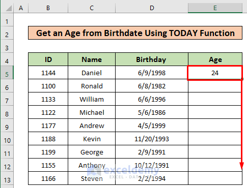
- Copy it down to E12.
- You will get the results like the following picture.
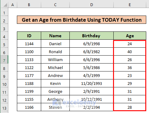
- YEAR(TODAY()) this portion extracts the year from the current date and YEAR(D4) which is from the birthday.
- Lastly, YEAR(TODAY())-YEAR(D4) this formula will determine the year differences.
Note:
- Make sure the Age column is in General Format.
Method 5 – Highlight Today’s Date in Excel Using the TODAY Function
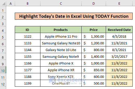
Now let’s see how we can highlight today’s dates.
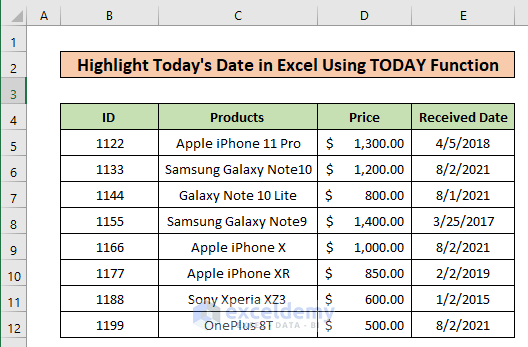
Steps:
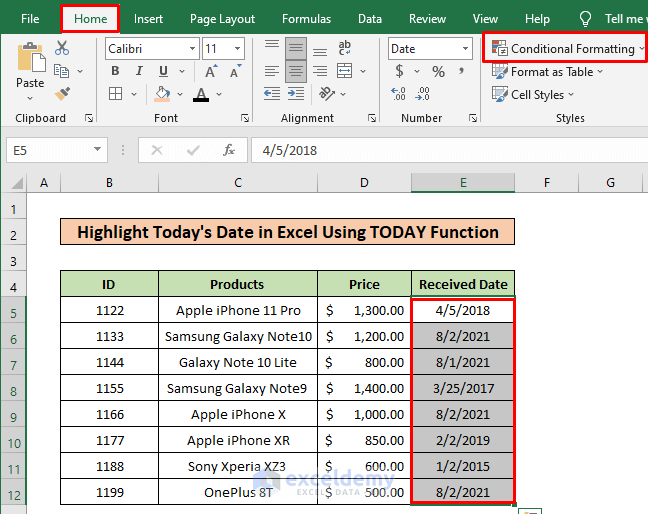
- Select the dates.
- Go to the Home tab and select Conditional Formatting under the Styles section.
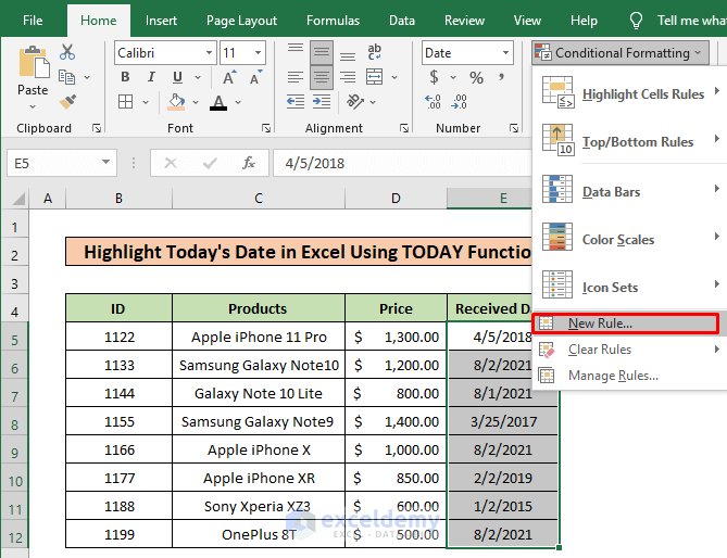
- Select the New Rules option
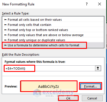
- Select the option to use a formula.
- Enter the following formula in the rule box.
=E4=TODAY()- Press the OK button.
- Here’s the result.
Method 6 – Get Any Date Closest to Today Using the TODAY Function
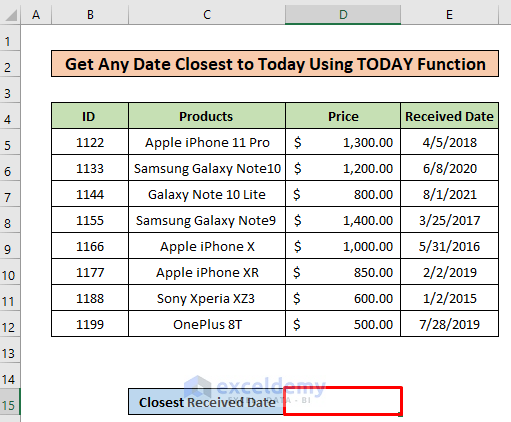
Let’s see how we can get the closest date from any dataset.
Steps:
- Enter the following formula in cell D14 and press Ctrl + Shift + Enter (As this is an array formula).
=INDEX($E$4:$E$11, MATCH(MIN(ABS($E$4:$E$11 - TODAY())), ABS($E$4:$E$11 - TODAY()), 0))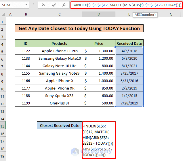
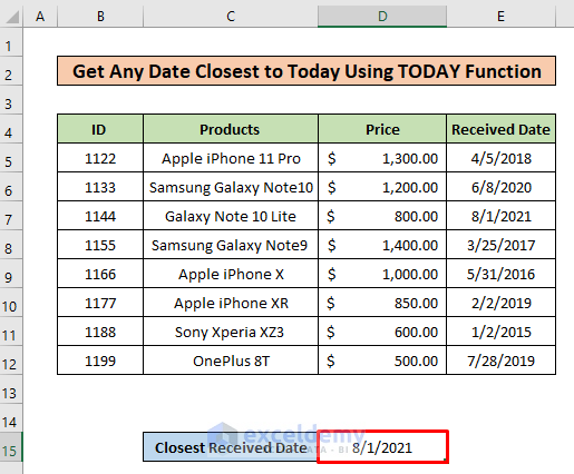
- After pressing Enter, you will get the following result.
How Does the Formula Work?
- ABS($E$4:$E$11 – TODAY()): This will find the difference between the given dates and today’s date and returns an absolute difference.
- MATCH(MIN(ABS($E$4:$E$11 – TODAY())): this sub-formula matches the minimum absolute difference.
- Lastly, $E$4:$E$11 is the data range where we will try to find the index value.
Shortcuts for the TODAY Function in Excel
- For Current Date
Ctrl + ;
- For Current Time
Ctrl + Shift + ;
- For Current Time
Ctrl + ; Space then Ctrl + Shift + ;
Things to Remember
- Make sure your cell is in the correct date format to use the TODAY function.
- If the start_date is formulated in an invalid format then, the EOMONTH function will return #VALUE! indicating an error in the value.
- Make sure your cells are in general format when you are calculating days, months, or years. Otherwise, it will return dates that are not correct for this kind of situation.
Download the Practice Workbook
<< Go Back to Excel Functions | Learn Excel
Get FREE Advanced Excel Exercises with Solutions!


I’m trying to do a countifs function that isn’t returning anything valid. And I believe it is with the Today function.
EXAMPLE: =countifs(D2:D9,[UIC],E2:E9,>TODAY())
If I do countif(D2:D9,[UIC]) it returns all that match the [UIC] like it should. When I add the second range and criteria, it’s failing.
Hello Katrina,
The issue lies in how COUNTIFS processes criteria. The function doesn’t accept logical operators directly without enclosing them in quotes. To fix the formula, modify it like this:
=COUNTIFS(D2:D9, “[UIC]”, E2:E9, “>” & TODAY())
1. [UIC] is a placeholder; ensure it matches values in D2:D9 or use a cell reference (e.g., A1).
2. “& TODAY()” ensures the date comparison is dynamically evaluated.
Double-check that E2:E9 contains valid dates and aligns with the D2:D9 range.
Regards
ExcelDemy