How to Calculate Total Row and Column in Excel: 4 Methods

Method 1 – Use the SUM Function to Calculate Total Row and Column in Excel

1.1 Calculate Total Row

Steps:

• Learn how to calculate row values from our dataset. Select a new cell. Select cell F5 and write down the SUM function in that cell. The SUM function is,

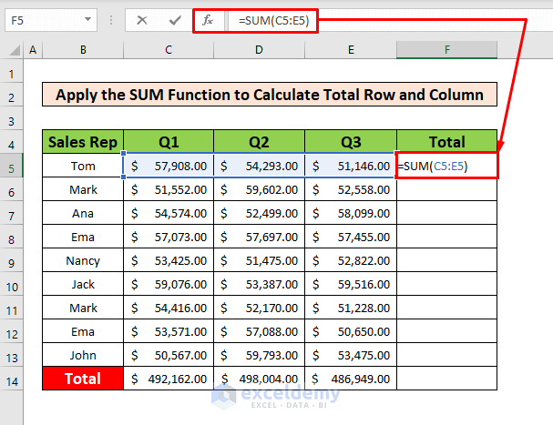
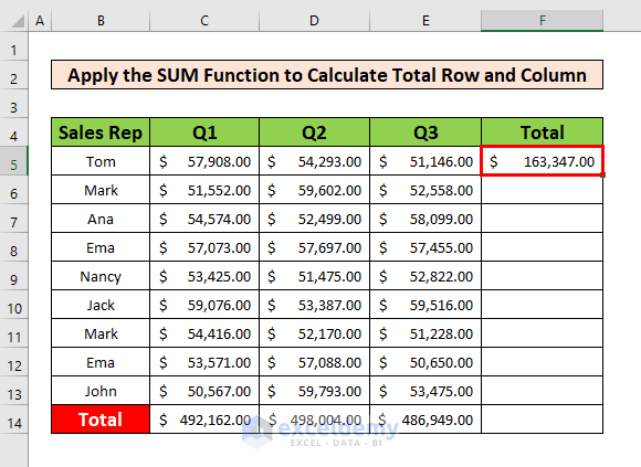
• Press Enter on your keyboard and you will be able to get $163,347.00 as the output of the SUM function.

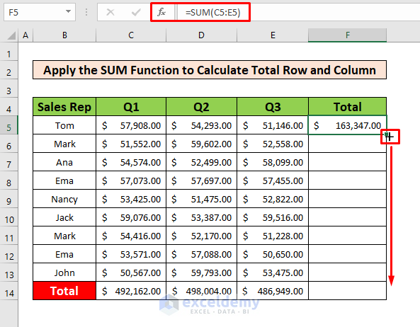
• Place your cursor on the bottom right side of cell F5 and an AutoFill sign pops up. Dag the AutoFill sign downward.

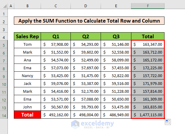
• After completing the above process, you will be able to get the output of the SUM function along with the rows shown in the screenshot below.

1.2 Calculate Total Column

Steps:

• Select cell C14, and type the SUM function to calculate the total sales in the first quarter in column C. The SUM function is,

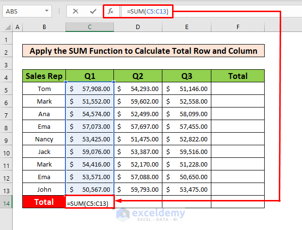
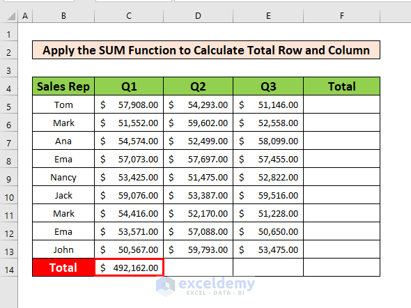
• After typing the SUM function in the Formula Bar, press Enter on your keyboard, and you will be able to get $492,162.00 as the return of the SUM function.

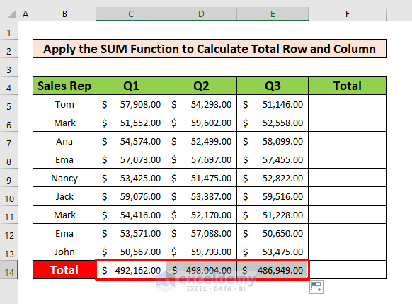
• AutoFill the SUM function in columns D, and E and you will get your desired output, which has been given in the below screenshot.

1.3  Non-contiguous Row and Column

Steps:

• Select cell E15.

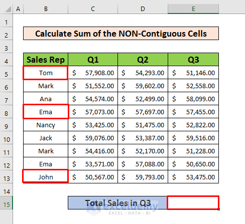
• Write down the SUM function in that cell.

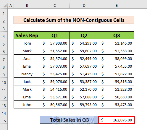
• Where E5 is the sales of Tom, E8 is the sales of Ema, and E13 is the sales of John in the 3rd quarter.

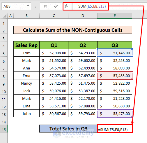
• Press Enter, and you will get your desired output as given in the screenshot below.

Method 2- nsert the AutoSum Formula to Calculate Total Row and Column in Excel

Step 1:

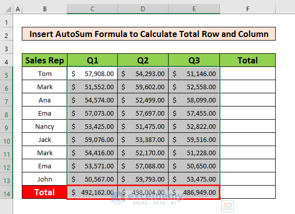
• Sum up cell values automatically by applying the AutoSum formula, first, select cells C5 to E13.

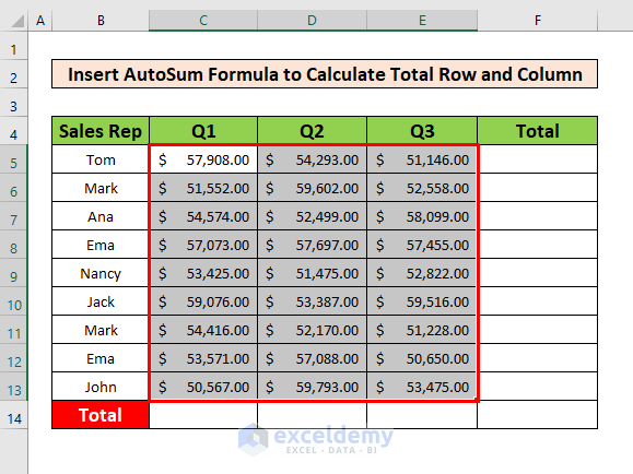
• From your Home Ribbon, go to

Home → Editing → AutoSum

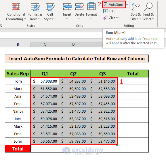
• Press on the AutoSum menu, and you will get the return of the AutoSum formula that has been given in the screenshot below.

Step 2:

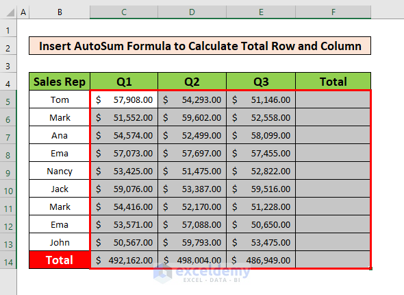
• Select rows 5 to 14 from our dataset.

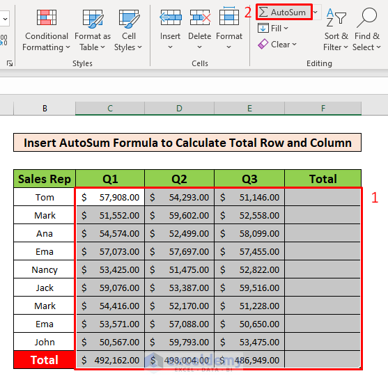
• From your Home Ribbon, go to

Home → Editing → AutoSum

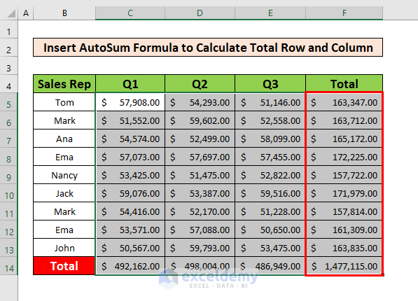
• Sum up, the total rows by using the AutoSum option.

Method 3 Apply the ROWS and COLUMNS Formula to Calculate Total Row and Column in Excel

Steps:

• Select cell H6, and type the COLUMNS function. Type in the Formula Bar is,

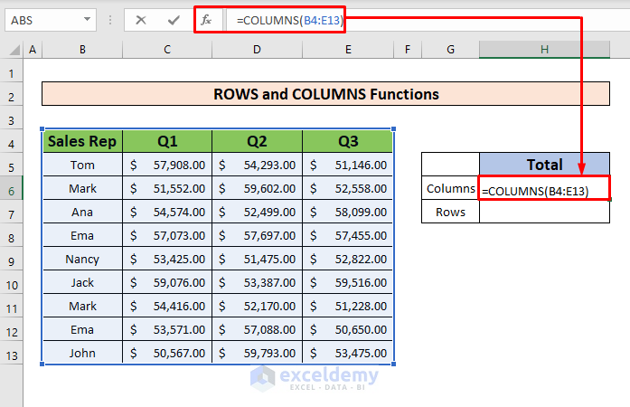
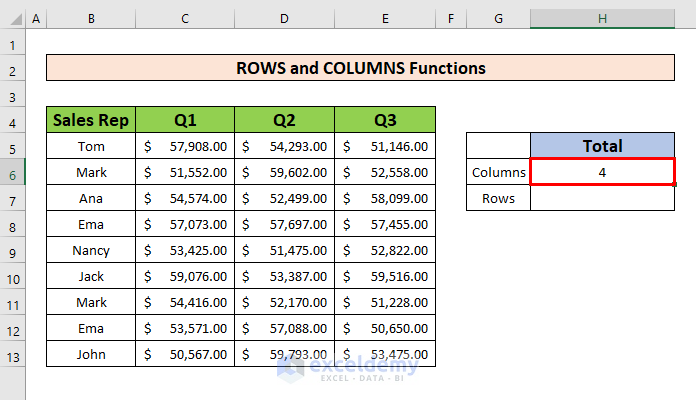
• After selecting cell H6, press Enter on your keyboard, and you will get 4 as the return of the COLUMNS function.

• Select cell H7 and write down the ROWS function. Type in the Formula Bar is

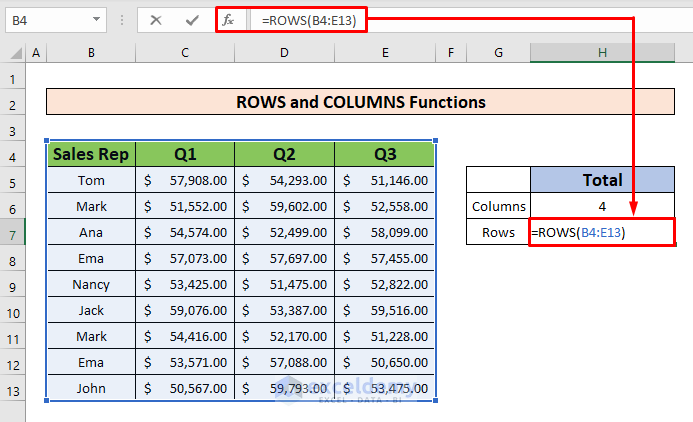
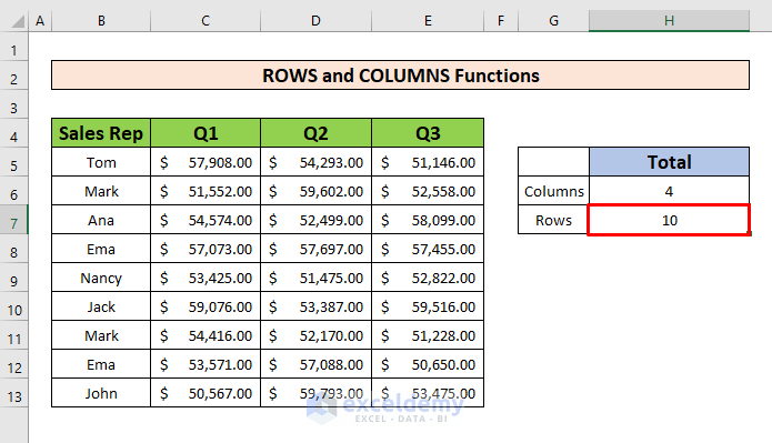
• Press Enter on your keyboard and you will get 10 as the output of the ROWS function.

Method 4 – Perform Table Design Option to Calculate Total Row and Column in Excel

Steps:

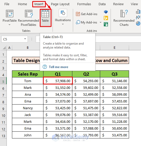
• Select any convenient cell for our work. Select cell C5 go to,

Insert → Tables → Table

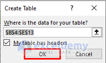
• While clicking on the Table option, a Creating Table window will instantly appear in front of you. From that window, press OK.

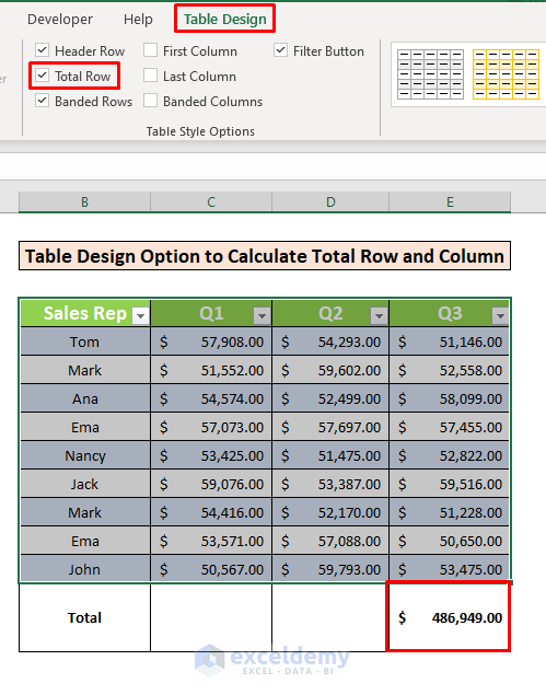
• From the Table Design ribbon, go to,

Table Design → Table Style Options → Total Row

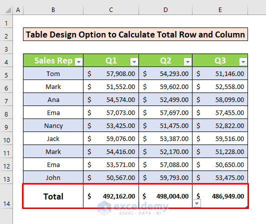
• Clicking on the Total Row, you will get the sum of column E in cell E14.

• Select cell C14, and a Filter Button will appear in the bottom right corner of that cell. Click the Filter Button, and a window will appear. From that window, select the Sum option.

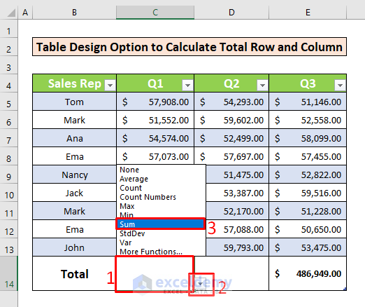
• Get $492,162.00 as the sum of column C in cell C14. Calculate the total sum of column D in cell D14 by performing the Table Design Option that has been given in the screenshot below.

Things to Remember

You can use Ctrl + Shift + T as keyboard shortcuts instead of the Table Design option. Another way to apply the AutoSum formula is Alt+=.

#NAME error will happen when the argument is not properly passed.

The error named #VALUE! happens when the value is not expected by the SUM function.

Download Practice Workbook

Download this practice workbook to exercise while you are reading this article.

Related Articles

• How to Sum Multiple Rows and Columns in Excel
• How to Sum Columns by Color in Excel 
• How to Sum Columns in Excel When Filtered 
• How to Sum Entire Column in Excel

<< Go Back to Sum Columns | Sum in Excel | Calculate in Excel | Learn Excel