Unhide All Rows Not Working in Excel (5 Issues & Solutions)

In this article, we’ll discuss 5 reasons why unhiding all rows is not working in Excel, and provide the solutions

Reason 1 – Freeze Panes is Enabled

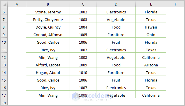
In the following picture, rows 1-5 are not visible.

The Unhide option for unhiding rows in the context menu has no effect.

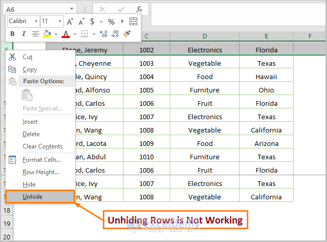
The reason is that Freeze Panes is enabled. Removing Freeze Panes will unhide the hidden rows.

STEPS:

• Go to the View tab.
• Click on the drop-down list of Freeze Panes and choose Unfreeze Panes.

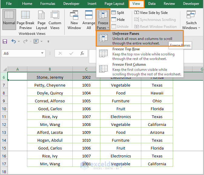
Note. The keyboard shortcut to unfreeze the panes: ALT + W + F  + F.

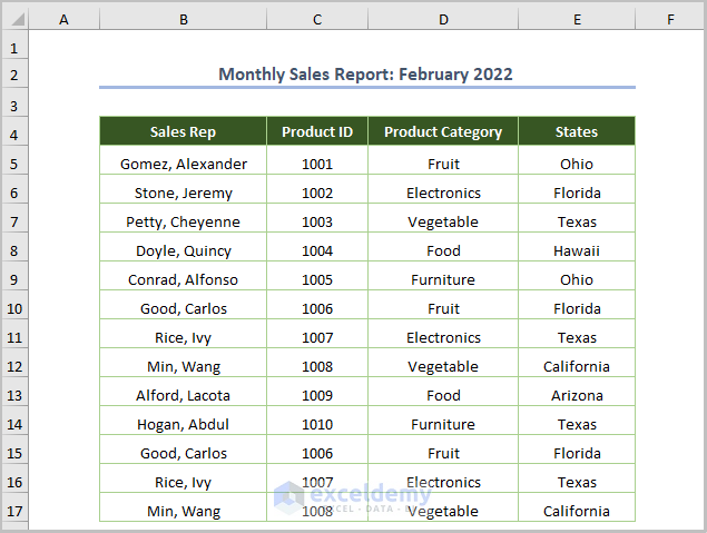
The unhidden rows are revealed, and the methods of hiding and unhiding rows will now work as expected.

Read More: VBA to Hide Rows Based on Cell Value in Excel

Reason 2 – Row Height is Very Small or Zero

Here, row 8 in the below image cannot be unhidden using the conventional methods of unhiding rows.

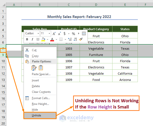
In fact, the row is not actually hidden, rather the row height is 0, which is why the unhiding it doesn’t work.

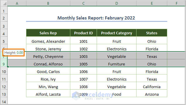
The same situation will occur if the row height is minuscule (between 0.08 and 0.67).

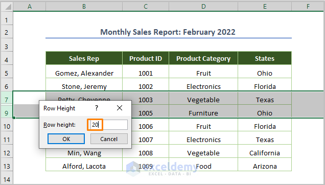
To solve the issue, simply increase the row height using the Row Height option from the Format menu (for example, to a height of 20).

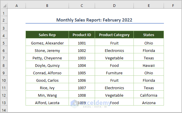
After increasing the row height, row 8 is visible again.

Reason 3 – Filter Mode is Active

In the following screenshot, Filter mode is active and Product IDs 1004 & 1005 are filtered out. As a result, rows 8-9 are not visible.

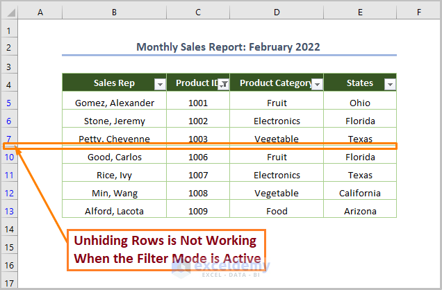
The only way to unhide the hidden rows is to remove the Filter.

STEPS:

• Go to the Data tab.
• Select Clear from the Filter option in the Sort & Filter section.

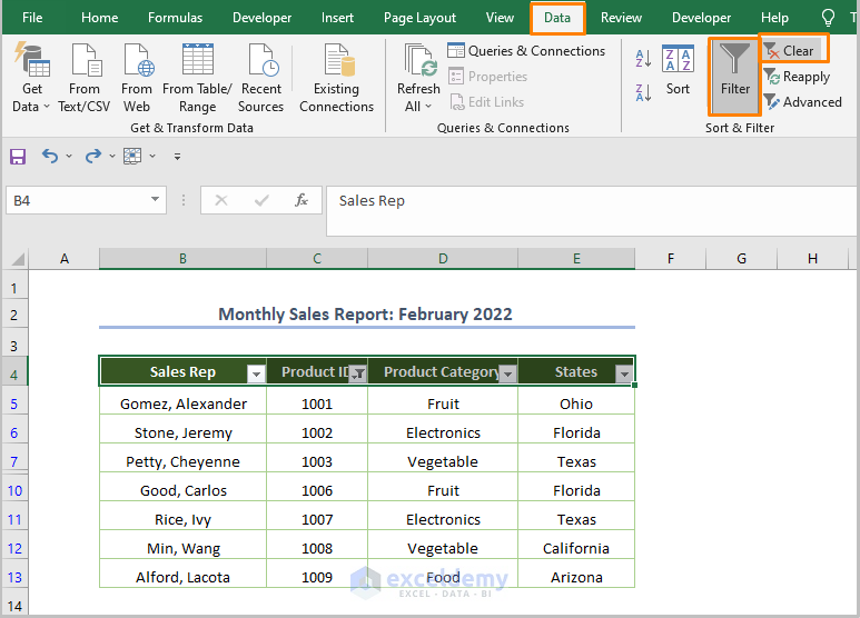
All filtered out / hidden rows are restored.

Read More: How to Unhide Rows in Excel

Reason 4 – The Sheet is Protected

Rows 7-10 in the following figure are not visible and cannot be unhidden using the Unhide Rows command.

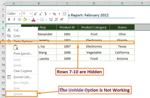
One possible reason is that sheet protection is active.

We can check whether it is protected or not using VBA.

STEPS:

• Open a module by clicking Developer > Visual Basic.

• Go to Insert > Module.

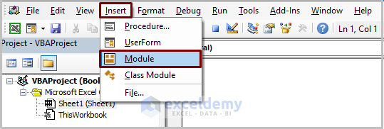
• Copy and the following code and paste it into the newly created module:

Sub SheetProtection()
If ActiveSheet.ProtectContents = True Then
MsgBox "The Sheet is Protected"
Else
MsgBox "The Sheet is Not protected"
End If
End Sub

• Run the code (the keyboard shortcut is F5 or Fn + F5).

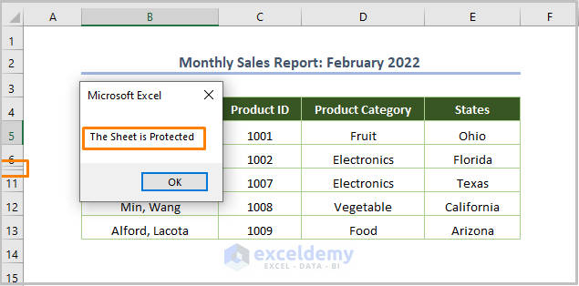
A message appears informing that “The Sheet is Protected”.

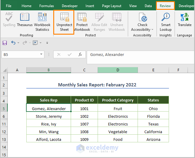
To unprotect the sheet:

• Go to the Review tab.
• Click on Unprotect Sheet from the Protect ribbon.

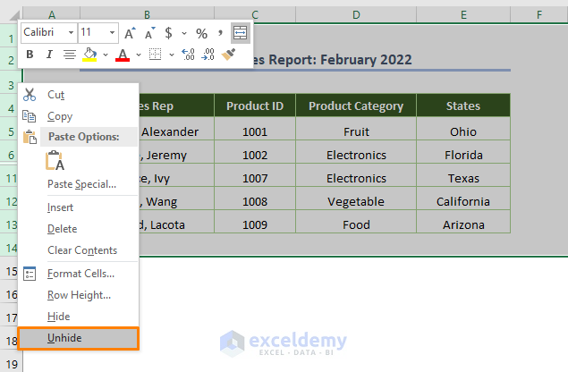
The Unhide option is available again in the context menu.

• Select the dataset, right-click on any cell, and select Unhide.

The hidden rows are visible again.

Reason 5 – Can’t Unhide the Top Row

The procedure for unhiding the top row of a worksheet is not the same as for other rows in Excel.

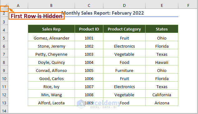
Unhiding the row from the context menu doesn’t work.

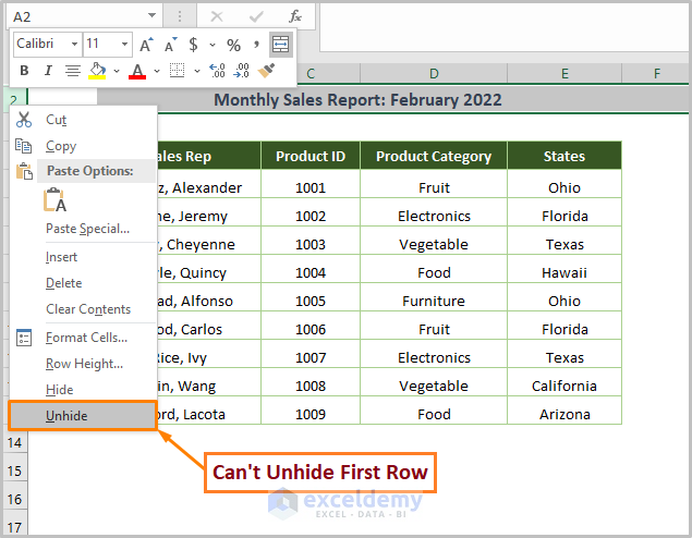
Here is the solution.

STEPS:

• Go to the Home tab
• Click on the Go To option from the Find & Select option in the Editing section.

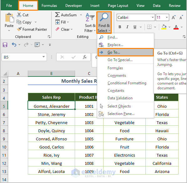
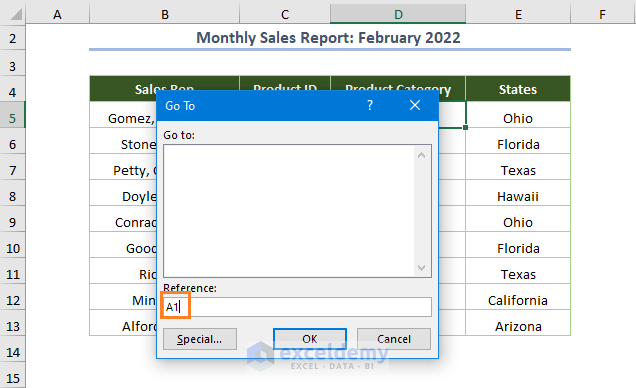
• Input A1 as the Reference and click OK.

• Click on the Unhide option from the context menu.

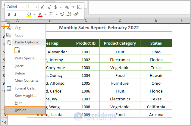
The hidden first row is visible.

Read More: Shortcut to Unhide Rows in Excel

Download Practice Workbook

Related Articles

• How to Unhide Top Rows in Excel
• [Fix]: Unable to Unhide Rows in Excel
• [Fixed!] Excel Rows Not Showing but Not Hidden

<< Go Back to Hide Rows | Rows in Excel | Learn Excel