How to Find Unique Values in an Excel Column (6 Methods)

Method 1 – Using Advanced Filter for Unique Values

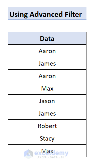
We’ll use the below dataset:

Steps

• Open your Excel workbook.

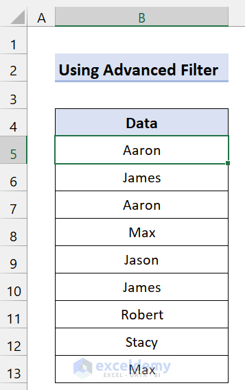
• Navigate to the Data tab.
• Look at the dataset you want to work with.
• Follow these steps:
  • Click on Advanced in the Sort & Filter group.

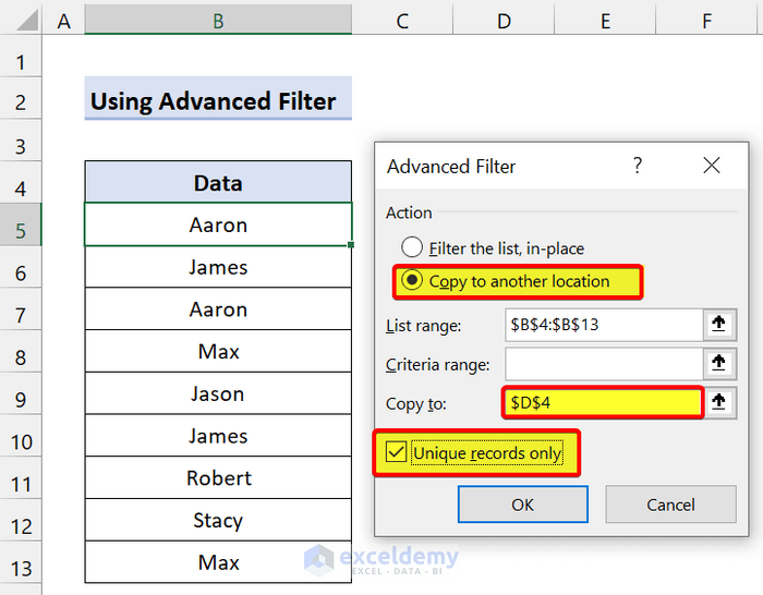
• • In the Advanced Filter dialog box, select Copy to another location.
  • Choose a cell where you want to paste the unique values.
  • Check the box for Unique records only.

• • Click OK.

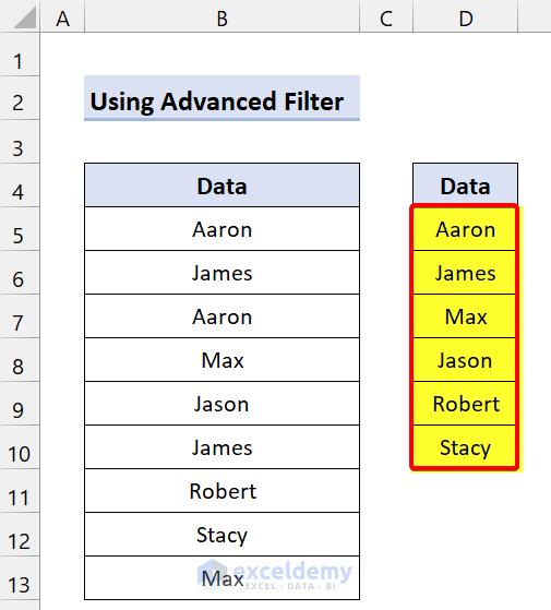
You’ve now created a new list of unique values from the selected column.

Method 2 -Filtering for Unique Values in a Column

Steps

• Select any cell within the column you want to filter.

• Go to the Data Tab.
• Click on Advanced in the Sort & Filter group.

• In the Advanced Filter dialog box:
  • Choose Filter the list, in-place.
  • Check the box for Unique records only.

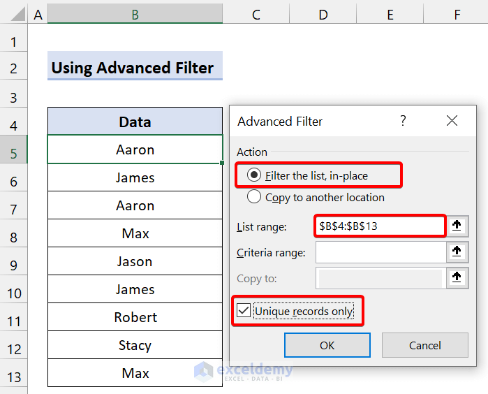
• Click OK.

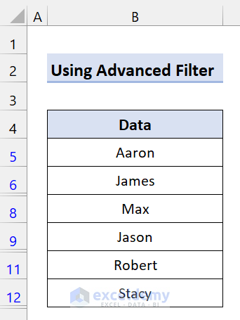
This method will display only the unique values in the column, effectively hiding any duplicate values.

Method 3 – Removing Duplicates from a Column

Steps

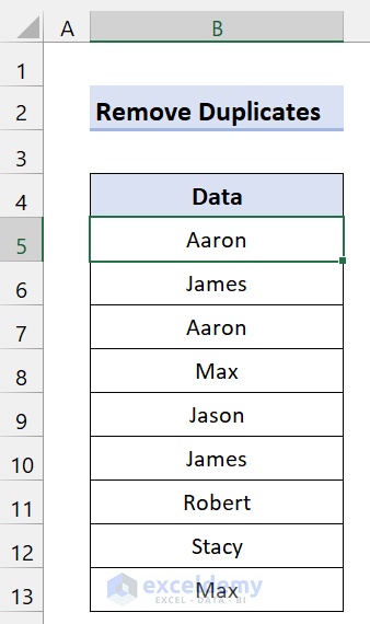
• Select any cell within the column containing duplicates.

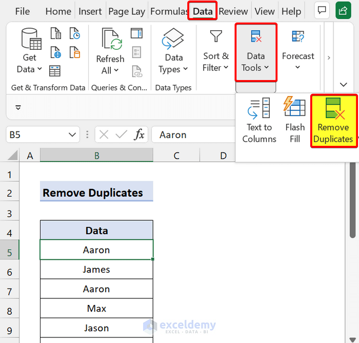
• Go to the Data tab.
• From the Data Tools group, click on Remove Duplicates.

• In the Remove Duplicates dialog box:
  • Ensure the box for Data is checked.
  • If your data has headers, check the box for My data has headers.

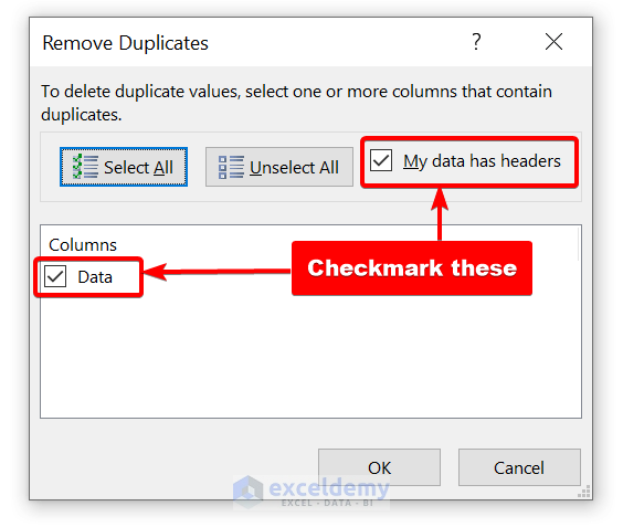
• Click OK.

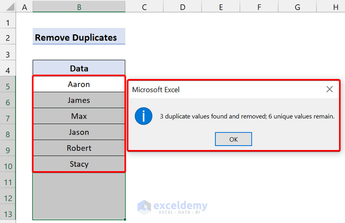
The result will show you how many duplicates were removed, leaving only the unique values in the column.

Method 4 – Formulas to Find Unique Values from a Column

You can use formulas to extract unique values from a column. These methods will also be useful in the future, so we recommend learning them to enhance your knowledge.

4.1 Using IF and COUNTIF Functions

Steps

• Create a new column.

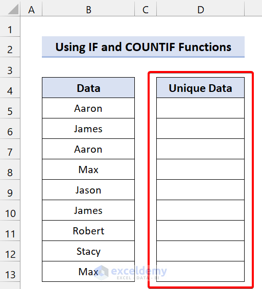
• In cell D5, enter the following formula:

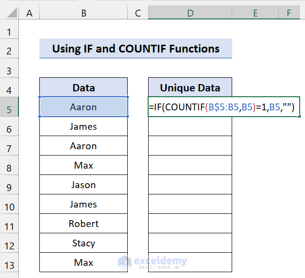
• Press Enter.
• Drag the Fill handle icon over the range of cells D6:D13.

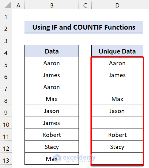
You’ll see that the column now contains only the unique values in Excel.

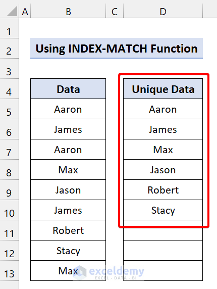
4.2 Using INDEX and MATCH Functions

Steps

• Create another new column.

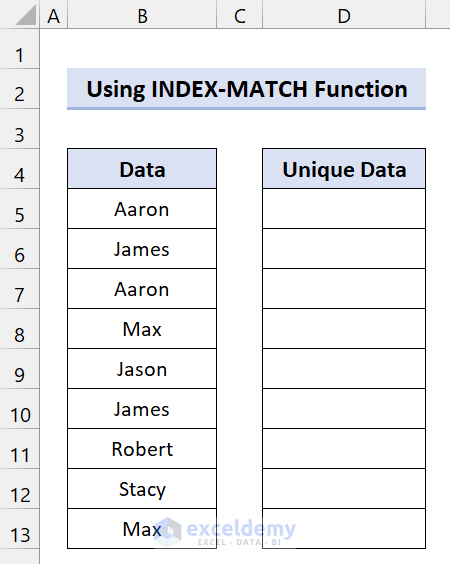
• In cell D5, enter the following formula:

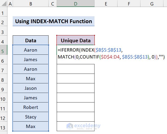
• Press Enter.
• Drag the Fill handle icon over the range of cells D6:D13.

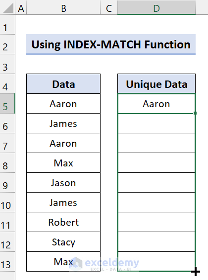
• This method allows you to easily extract unique values from an Excel cell.

Method 5 – Using the UNIQUE Function in Excel

The UNIQUE function in Excel is an essential method for finding unique values in a column. It returns a list of distinct values from a specified range or list. You can use it to extract both unique and distinct values, as well as compare columns or rows.

5.1 Extracting Unique Values from a Column

Steps

• Create a new column.

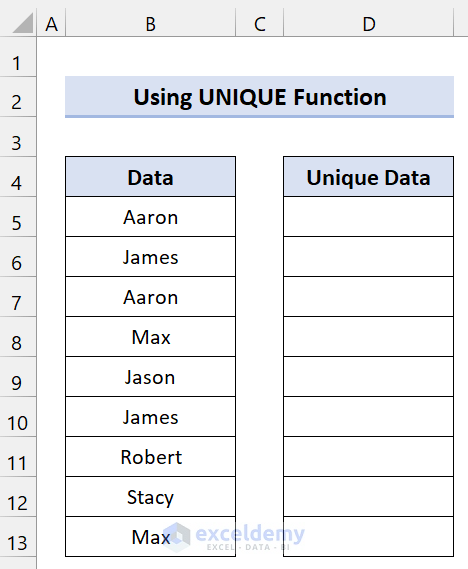
• In cell D5, enter the following formula:

• Press Enter.

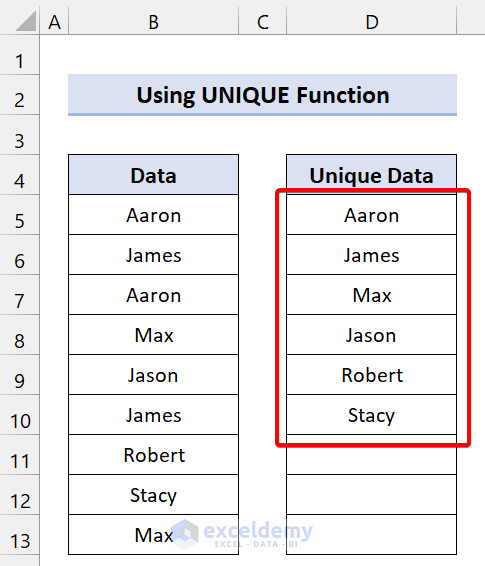
The result will be a list of all unique values from the specified column.

5.2 Extracting Unique Values with Only One Occurrence

Some values occur multiple times in the column, while others appear only once. These unique values with a single occurrence are particularly interesting. To find them, set the third argument of the UNIQUE function to TRUE.

Steps

• Create another new column as per the below example.

• In cell D5, enter the following formula:

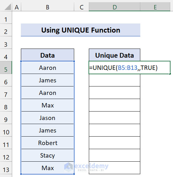
• Press Enter.

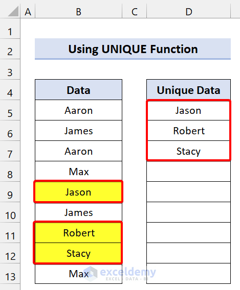
You’ll see that only three unique values appear once in the column.

5.3 Extracting Unique Values from Multiple Columns

You can also use the UNIQUE function on multiple columns that contain unique rows. It returns an array of unique values from the specified columns.

For example, if you have data in columns B and C, follow these steps:

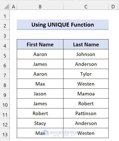
Steps

• Enter the following formula in Cell E5:

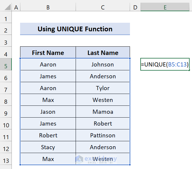
• Press Enter.

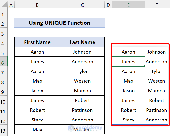
The result will be a list of unique values from both columns B and C.

5.4 Sorting Unique Values in Alphabetical Order

You can extract unique values from a column in alphabetical order using the SORT function. Unlike the manual sort and filter command, this method automatically arranges the data for you.

Steps

• Create a new column.

• In cell D5, enter the following formula:

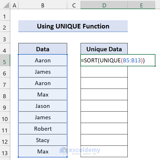
• Press Enter.

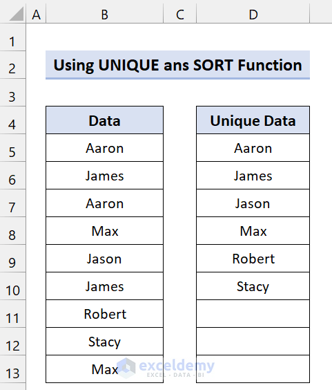
The result will be a list of unique values sorted alphabetically in the new column.

5.5 Finding Unique Values Based on Criteria

To find unique values based on specific criteria in Excel, combine the UNIQUE function with the FILTER function.

Example: Suppose you have a dataset with columns B (values) and C (ages). You want to find unique values where the age is less than 30.

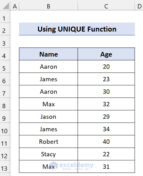
Steps

• Create two new columns.

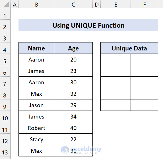
• In cell D5, enter the following formula:

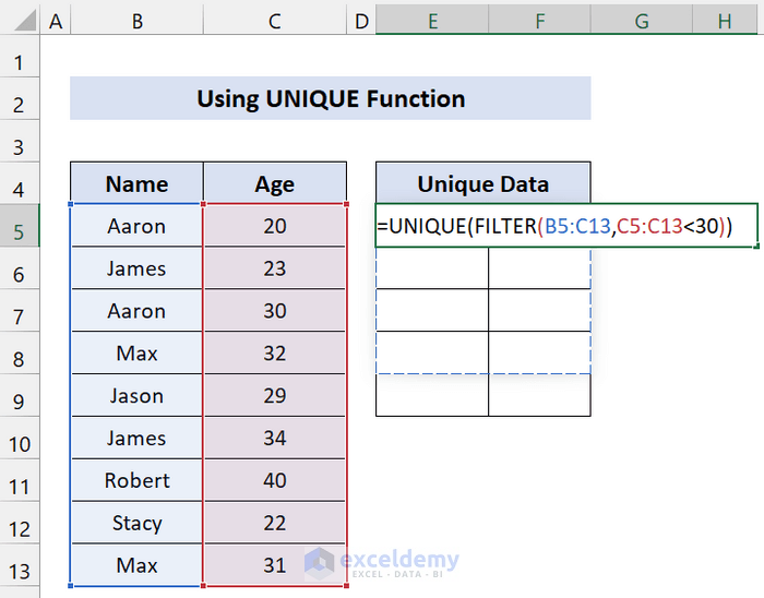
• Press Enter.

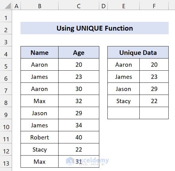
The result will display unique values from column B where the corresponding age in column C is less than 30.

Method 6 – VBA Macros for Unique Values in a Column

If you’re familiar with VBA (Visual Basic for Applications), you can create a new column with unique values using a VBA macro. This method is similar to the Advanced filter approach but automates the process.

Steps

• Press Alt+F11 to open the Visual Basic Application.
• Click on Insert and select Module.

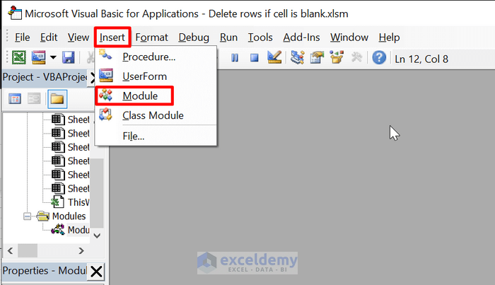
• Enter the following code:

Option Explicit
Sub UniqueColumn()
Dim last_row As Long
last_row = Cells(Rows.Count, "B").End(xlUp).Row
ActiveSheet.Range("B2:B" & last_row).AdvancedFilter _
Action:=xlFilterCopy, _
CopyToRange:=ActiveSheet.Range("D2"), _
Unique:=True
End Sub

• Save the file.
• Press Alt+F8 to open the Macro dialog box.

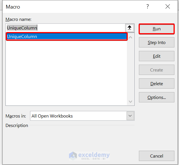
• Select UniqueColumn and click Run.

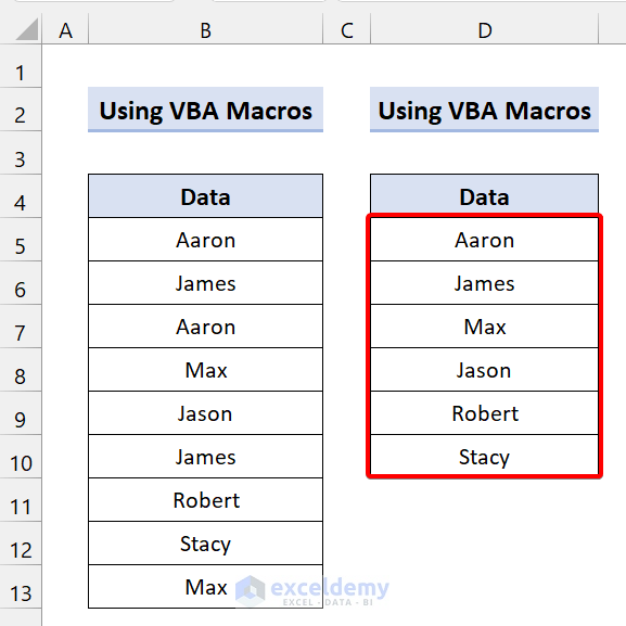
Your VBA code will successfully create a new column with unique values in Excel.

Things to Remember

• Understanding UNIQUE Function:
  • The examples provided here demonstrate basic usage of the UNIQUE function. For a more comprehensive understanding, consider reading the article we mentioned.
  • The UNIQUE function returns a list of distinct values from a specified range or list.
• #SPILL Error:
  • Be aware that the UNIQUE function may display a #SPILL error if one or more cells within the spill range are not blank. Ensure that your data meets the necessary criteria for successful execution.
• Data Overwriting:
  • If you want to preserve your original data, create a copy before applying the UNIQUE function. This way, you won’t accidentally overwrite your existing information.

Download Practice Workbook

You can download the practice workbook from here:

<< Go Back to Learn Excel