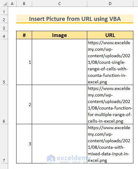
How to Insert Picture from URL Using VBA in Excel (2 Methods)

We will use the sample dataset below to insert images into the blank column (Image column) from the URLs given in the URL column.

Method 1 – Using VBA to Insert Picture from URL in Excel

Steps:

From the Developer tab >>> select Visual Basic.

The Visual Basic window will open.

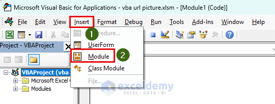
From Insert >>> select Module.

Enter the following code into the Module.

Sub URLPhotoInsert()
    Dim cShape As Shape
    Dim cRange As Range
    Dim cColumn As Long
    On Error Resume Next
    Application.ScreenUpdating = False
    Set xRange = ActiveSheet.Range("D5:D10")
    For Each cell In xRange
        cName = cell
        ActiveSheet.Pictures.Insert(cName).Select
        Set cShape = Selection.ShapeRange.item(1)
        If cShape Is Nothing Then GoTo line22
        cColumn = cell.Column - 1
        Set cRange = Cells(cell.Row, cColumn)
        With cShape
            .LockAspectRatio = msoTrue
            If .Width > cRange.Width Then .Width = cRange.Width * 3 / 4
            If .Height > cRange.Height Then .Height = cRange.Height * 3 / 4
            .Top = cRange.Top + (cRange.Height - .Height) / 2
            .Left = cRange.Left + (cRange.Width - .Width) / 2
        End With
line22:
        Set cShape = Nothing
        Range("D5").Select
    Next
    Application.ScreenUpdating = True
End Sub

VBA Code Breakdown

On Error Resume Next
- If the code finds any Runtime Errors, it will go to the next statement.
Application.ScreenUpdating = False
- The ScreenUpdating property is set to False to speed up the macro execution speed.
Set xRange = ActiveSheet.Range(“D5:D10”)
- Our URL range is up to cell D7, but we’ve set it to D5:D10 to demonstrate that it will work in the case of an empty cell. You need to change this based on your data.

We’re running a “For loop” within that URL cell range.

cColumn = cell.Column – 1
- The picture is set to be inserted in the C column (before the image URL). You need to change it accordingly.

If there is a blank cell, line 22 will be executed. The picture properties is set in the With cShape portion.

.LockAspectRatio = msoTrue
- The picture aspects ratio is set to be in a locked state.

If the picture is larger than the cell size, the width and the height are also set to 75% of the cell size.

Then close the window.

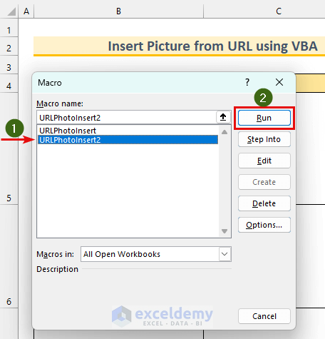
From the Developer tab >>> select Macros.

The Macro dialog box will pop up.

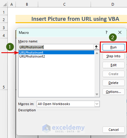
Select “URLPhotoInsert” as “Macro name:”.
Click on Run.

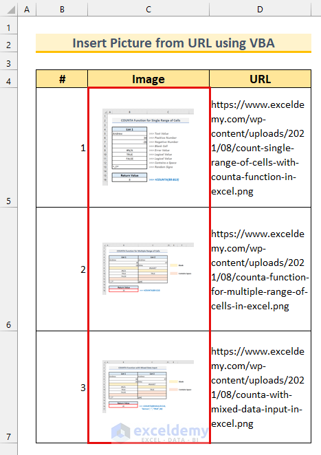
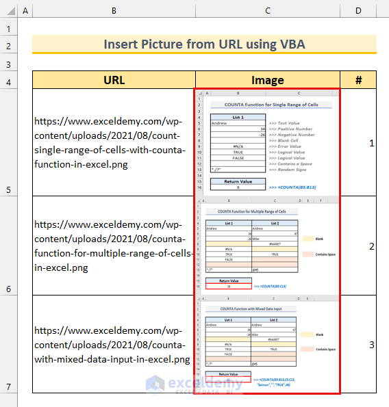
The pictures will appear in the middle column. If you have a large number of picture URLs, it may take a longer time.

Method 2 – Using the Range.Offset Property to Insert Picture from URL

Here, we’ll insert pictures from the URL using Excel VBA in the cell range C5:C7. Here, we’ll use the Range.Offset property to choose the picture location in our sheet.

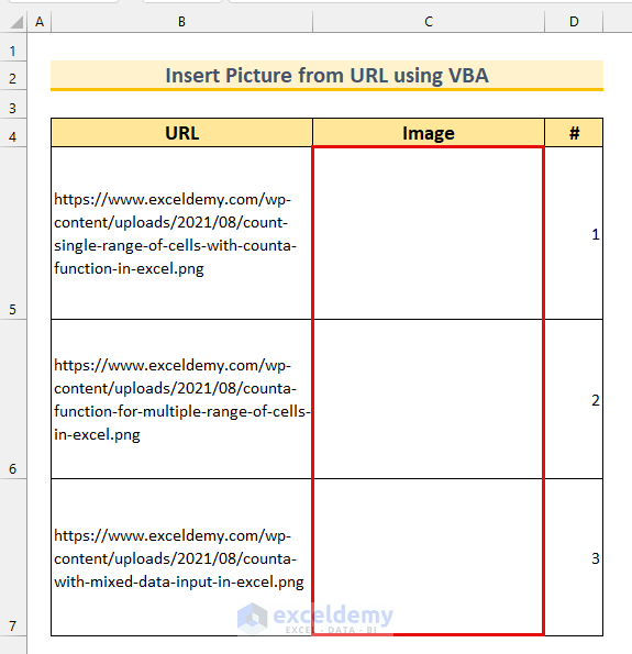
Steps:

Follow the steps from method 1 to open the VBA module.
Enter the following code in that Module:

Sub URLPhotoInsert2()
Dim cPhoto As String
Dim cPicture As Picture
Dim cRange As Range
Dim cItem As Range
Set cRange = Range("C5:C10")
For Each cItem In cRange
    cPhoto = cItem.Offset(0, -1)
    If cPhoto = "" Then Exit Sub
        Set cPicture = ActiveSheet.Pictures.Insert(cPhoto)
        With cPicture
            .ShapeRange.LockAspectRatio = msoFalse
            .Width = cItem.Width
            .Height = cItem.Height
            .Top = Rows(cItem.Row).Top
            .Left = Columns(cItem.Column).Left
            .Placement = xlMoveAndSize   
        End With 
    Next
End Sub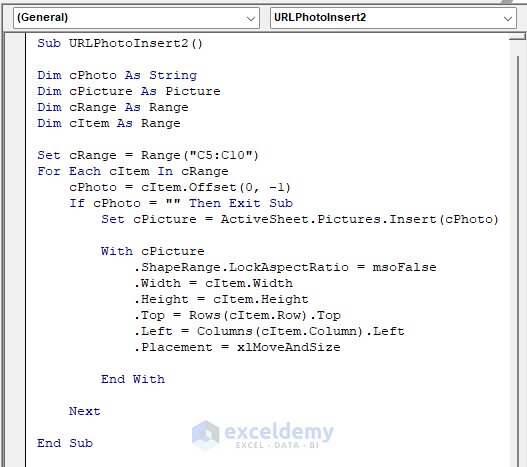

VBA Code Breakdown

Set cRange = Range(“C5:C10”)
- The cell range is set to C5:C10. Empty cells were added to prove that our code works in the case of an empty cell. This is the cell range where the picture will be inserted. You need to change it for your dataset.
cPhoto = cItem.Offset(0, -1)
- This command is to get the picture URL from the B column.

The picture properties are adjusted using the With cPicture portion.

.ShapeRange.LockAspectRatio = msoFalse
- We’re not locking the aspect ratio of the picture.
.Placement = xlMoveAndSize
- This ensures the picture moves and resizes with the cell.

Save and close the window.
Open the Macro window.
Choose “URLPhotoInsert2”.
Click on Run.

The pictures will be inserted in column C.

Download Practice Workbook

Insert Picture from URL Using VBA.xlsm

Get FREE Advanced Excel Exercises with Solutions!

Sub URLPhotoInsert2() Dim cPhoto As String Dim cPicture As Picture Dim cRange As Range Dim cItem As Range Set cRange = Range("C5, C8, C11") For Each cItem In cRange cPhoto = cItem.Offset(0, -1) If cPhoto = "" Then Exit Sub Set cPicture = ActiveSheet.Pictures.Insert(cPhoto) With cPicture .ShapeRange.LockAspectRatio = msoFalse .Width = cItem.MergeArea.Width .Height = cItem.MergeArea.Height .Top = Rows(cItem.Row).Top .Left = Columns(cItem.Column).Left .Placement = xlMoveAndSize End With Next End Sub

Sub URLPhotoInsert2() Dim cPhoto As String Dim cPicture As Shape Dim cRange As Range Dim cItem As Range Set cRange = Range("C5:C10") For Each cItem In cRange cPhoto = cItem.Offset(0, -1) If cPhoto = "" Then Exit Sub Set cPicture = ActiveSheet.Shapes.AddPicture(cPhoto, _ msoFalse, msoTrue, Columns(cItem.Column).Left, _ Rows(cItem.Row).Top, cItem.Width, cItem.Height) With cPicture .LockAspectRatio = msoFalse .Placement = xlMoveAndSize End With Next End Sub

Sub URLPhotoInsert2() Dim cPhoto As String Dim cPicture As Picture Dim cRange As Range Dim cItem As Range Set cRange = Range("C5:C10") For Each cItem In cRange cPhoto = cItem.Offset(0, -1) If cPhoto = "" Then GoTo line33 Set cPicture = ActiveSheet.Pictures.Insert(cPhoto) With cPicture .ShapeRange.LockAspectRatio = msoFalse .Width = cItem.Width .Height = cItem.Height .Top = Rows(cItem.Row).Top .Left = Columns(cItem.Column).Left .Placement = xlMoveAndSize End With line33: cPhoto = "" Next End Sub

Sub Keeping_Aspect_Ratio_Constant() Dim cPhoto As String Dim cPicture As Picture Dim cRange As Range Dim cItem As Range Set cRange = Range("C5:C7") For Each cItem In cRange cPhoto = cItem.Offset(0, -1) If cPhoto = "" Then GoTo line33 Set cPicture = ActiveSheet.Pictures.Insert(cPhoto) With cPicture .ShapeRange.LockAspectRatio = msoTrue .Width = cItem.Width If .Height > cItem.Height Then .Height = cItem.Height .Top = Rows(cItem.Row).Top + (Rows(cItem.Row).Height - .Height) / 2 .Left = Columns(cItem.Column).Left + (.TopLeftCell.Width - .Width) / 2 .Placement = xlMoveAndSize End With line33: cPhoto = "" Next End Sub

Option Explicit Sub URLPhotoInsert2() Dim cPhoto As String Dim cPicture As Shape Dim cRange As Range Dim cItem As Range Set cRange = Range("C5:C10") For Each cItem In cRange cPhoto = cItem.Offset(0, -1) If cPhoto = "" Then GoTo line33 Set cPicture = ActiveSheet.Shapes.AddPicture(cPhoto, _ msoFalse, msoTrue, Columns(cItem.Column).Left, _ Rows(cItem.Row).Top, -1, -1) If cPicture.Width > cItem.Width Then cPicture.Width = cItem.Width If cPicture.Height > cItem.Height Then cPicture.Height = cItem.Height With cPicture .Top = Rows(cItem.Row).Top + (Rows(cItem.Row).Height - .Height) / 2 .Left = Columns(cItem.Column).Left + (.TopLeftCell.Width - .Width) / 2 .LockAspectRatio = msoTrue .Placement = xlMoveAndSize End With line33: cPhoto = "" Next End Sub

24 Comments

dimas May 13, 2022 at 9:01 PM

how to modify this code if i have merged range? as an example:
Set cRange = Range(“C5:C7, C8:C10, C11:C13”)

This code successfully retrieves the first value (URL) from the merged range, but the image position is only in the range C5, C8, and C11. What I want is the image position to be at C5:C7, C8:C10, C11:C13.
- Reply
  Rafiul Haq May 14, 2022 at 11:35 PM
  According to your example, Set cRange = Range(“C5, C8, C11”)
  Then, you’ll need to change the height & width to MergeArea
  .Width = cItem.MergeArea.Width
  .Height = cItem.MergeArea.Height
  
  Full Code >
```
Sub URLPhotoInsert2()
Dim cPhoto As String
Dim cPicture As Picture
Dim cRange As Range
Dim cItem As Range
Set cRange = Range("C5, C8, C11")
For Each cItem In cRange
    cPhoto = cItem.Offset(0, -1)
    If cPhoto = "" Then Exit Sub
        Set cPicture = ActiveSheet.Pictures.Insert(cPhoto)
        With cPicture
            .ShapeRange.LockAspectRatio = msoFalse
            .Width = cItem.MergeArea.Width
            .Height = cItem.MergeArea.Height
            .Top = Rows(cItem.Row).Top
            .Left = Columns(cItem.Column).Left
            .Placement = xlMoveAndSize
        End With
    Next
End Sub
```
  The output will be this: https://ibb.co/KXHVzSC
  - Reply
    Suzanna Cocker Sep 19, 2024 at 3:33 PM
    
    Hi Rafiul, Thank you so much for adding this guide it has been so useful for me to be able to make use of as when I tried using a different guide someone else had done it didnt work for me but yours works perfect! Just one quick question, do you happen to have a guide on how to remove the pictures too once they have been added? I have created a button within my spreadsheet and assigned the macro code to add the pictures, but would also like to be able to remove them easily rather than having to do it manually one by one!
    Thanks Suzanna
    - Shamima Sultana Sep 23, 2024 at 12:23 PM
      
      Hello Suzanna Cocker,
      
      You are most welcome. Thanks for your appreciation. To remove the pictures added via VBA, you can create another macro assigned to a button to delete them. Copy paste the VBA code that will remove all the shapes (including images) from the sheet.
      
      Sub RemovePictures() Dim Pic As Shape For Each Pic In ActiveSheet.Shapes If Pic.Type = msoPicture Then Pic.Delete End If Next Pic End Sub
      
      This code will delete all pictures in the active sheet when the button is clicked. You can add this to your existing setup.
      
      Regards
      ExcelDemy
  - Reply
    Robin Jul 27, 2022 at 2:39 AM
    
    I want to send the file, but the images disappear when saving. How to save the loaded images in the file?
    - Rafiul Haq Jul 28, 2022 at 6:27 PM
      
      Thank you for your question.
      
      In my second code, instead of “ActiveSheet.Pictures.Insert” you can try using “ActiveSheet.Shapes.AddPicture”, which should embed the images in the Excel file and it will not disappear.
      
      the modified VBA code from the second method will be:
      
      Sub URLPhotoInsert2() Dim cPhoto As String Dim cPicture As Shape Dim cRange As Range Dim cItem As Range Set cRange = Range("C5:C10") For Each cItem In cRange cPhoto = cItem.Offset(0, -1) If cPhoto = "" Then Exit Sub Set cPicture = ActiveSheet.Shapes.AddPicture(cPhoto, _ msoFalse, msoTrue, Columns(cItem.Column).Left, _ Rows(cItem.Row).Top, cItem.Width, cItem.Height) With cPicture .LockAspectRatio = msoFalse .Placement = xlMoveAndSize End With Next End Sub
Milagros Huerta Jun 13, 2022 at 4:19 AM

Does it work with images in Google Drive shared with those who have the link? I’m trying but I can’t.

It also doesn’t work for me with the following image:
https://www.exceleinfo.com/wp-content/uploads/2022/06/Referencias-3D-en-Excel-1024×477.png

It works fine with this image:
https://sea-eu.org/wp-content/themes/theme_seaeu_uca/images/logo/logo_seaeu4.png

I do not know what I’m doing wrong
- Reply
  Rafiul Haq Jul 18, 2022 at 10:35 PM
  
  You need to change Google Drive’s Shared URL when inputting it into the cell.
  For example, if I share an image the URL will be -> “https://drive.google.com/file/d/18r34oAVY8-bicTmf3CaTIumuHp_hqZxH/view?usp=sharing”.
  Then, I need to change it to -> “https://drive.google.com/uc?export=view&id=18r34oAVY8-bicTmf3CaTIumuHp_hqZxH” (putting the values after d/ inside the id values of the URL).
  
  And for your second question, I think the URL is not correct, if I remove the image resolution info from the URL, then it works perfectly in my second code.
  
  Your URL -> “https://www.exceleinfo.com/wp-content/uploads/2022/06/Referencias-3D-en-Excel-1024×477.png”.
  it should be -> “https://www.exceleinfo.com/wp-content/uploads/2022/06/Referencias-3D-en-Excel.png”.

Amilia Aug 22, 2022 at 1:18 PM

Hi Raiful,
Thanks for sharing this!
But I have 1 problem with this. I used the excel data from Ms. Form and some rows don’t have any image URL since they didn’t upload image on the form. When I applied your second way of attaching image, it stopped to insert image if the cell is empty, but the row below that also stopped working (stopped attaching the image as well).
Could you please help me?

Thanks in advance.

Rafiul Haq Aug 24, 2022 at 2:17 PM

Hello Amilia. Thank you for your question. You can use the following VBA code to ignore blank cells within the range.

Amilia Aug 22, 2022 at 4:16 PM

Hi! How to make command that if the cell is empty, it will go to the next cell and so on until the end of the cell range? Thanks!
- Reply
  Rafiul Haq Aug 24, 2022 at 2:24 PM
  
  I have modified the VBA code from the second method to handle blank cells for your dataset. Please check the solution to your first comment.

Robin Oct 22, 2022 at 6:54 PM

Hello,

Currently pictures which are high and a have a small width are pulled completely out of proportion. Is it possible to keep the proportions of the picture and fit within the cell?

Rafiul Haq Oct 22, 2022 at 10:21 PM

You can use this code to keep the image proportion.

Here is the output.

Robin Oct 24, 2022 at 4:29 PM

Hi,

That’s great! And how do I combine it with the earlier solution you gave for saving the images within the file?

Rafiul Haq Oct 31, 2022 at 5:59 PM

Hello Robin. This code should work for you. It will make the image fit in the output cell, keep the aspect ratio constant, and the image will not disappear.

Andreas Oct 30, 2022 at 4:10 PM

Hey – thank you very much for this pedagogical description.

I have a question regarding a Twitter scribing I’m conducting, where I would like to convert the media_URLs into photo. It works regarding the photo whose URL is still active. But some of the others doesn’t. Then I get a box saying “File not found: The file that you’re trying to insternt is no longer available”. I can manually click on the message box each time. But if’ I’m getting excel to converting a data set <1000 URL's and half of them needs me to click. Is there any way in the VBA script that this can be automated?

Best regards
Andreas
- Reply
  Rafiul Haq Oct 31, 2022 at 9:24 AM
  Hello Andreas, you need to add the following line to ignore the error.
```
On Error Resume Next
```
Anwer Jan 10, 2023 at 12:59 PM

Hi Im trying the code but could not success, though have followed the steps carefully even enabled macro too but your code no functioning im my excel sheet.
- Reply
  Fahim Shahriyar Dipto Jan 11, 2023 at 2:31 PM
  
  Hello Anwer,
  Thanks for your comment. It is the most common factor when you download a .xlsnm, the code doesn’t work. So, to avoid this consequence follow the steps stated below.
  Firstly, download the .xlsm file from the article and right-click on the file. Select Properties.
  
  Then, check the Unblock box and hit OK.
  
  Hopefully, this method solves your issue. If not then change the directory of the file and Rename it at your preference. then the VBA code of the source file will run in the existing worksheet.
  Again, if you are facing any obstacle then mail the Excel file to the address.
  Regards,
  Fahim Shahriyar Dipto
  Excel & VBA Content Developer
Nesreen May 20, 2023 at 1:48 AM

Hello

I tried your code .. It works well for some JPG images but some other JPG images Url are not displayed.. It doesn’t give me an error but just doesn’t display the images ..

Thanks in advance
Sishir Roy May 21, 2023 at 1:36 PM

Hello NESREEN,
I wanted to inform you that the code mentioned in the first method of the provided article has been executed successfully, and the images have been inserted into the designated range using the provided URLs.

If you experience any difficulties, please double-check that you copied the URLs accurately and that the range you chose is accurate. Also if you need further assistance, please don’t hesitate to share your concerns or provide the Excel file for a more detailed analysis. If any URL doesn’t work, you can share the URL with us also.

Thank you for your cooperation. We are here to help and ensure a smooth experience.

Best Regards,
Sishir Roy
Juan Nov 21, 2023 at 9:22 PM

Beatiful code.
Thanks a lot!!!
- Reply
  Shamima Sultana Nov 22, 2023 at 9:02 AM
  
  Hello Juan,
  
  You are most welcome.
  
  Regards
  ExcelDemy

How to Insert Picture from URL Using VBA in Excel (2 Methods)

Method 1 – Using VBA to Insert Picture from URL in Excel

Method 2 – Using the Range.Offset Property to Insert Picture from URL

Related Articles

Leave a reply Cancel reply