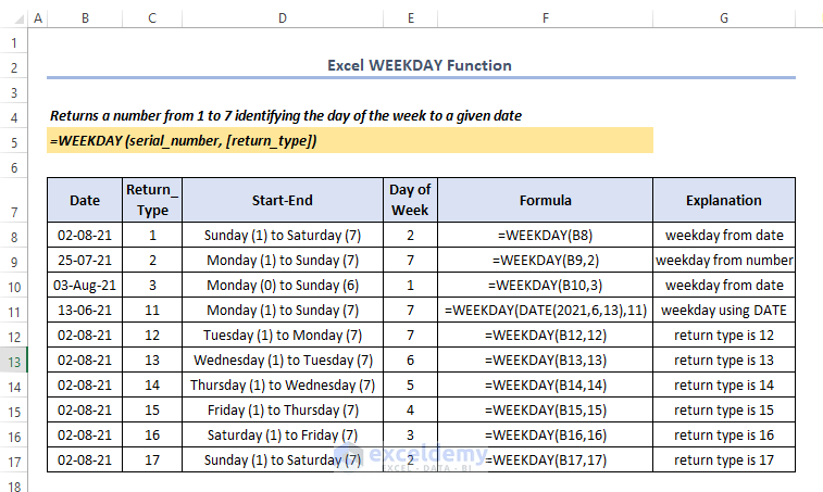
Excel WEEKDAY Function: Syntax & Arguments
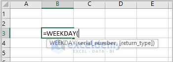
Syntax
Return Values
0 to 7 (in numbers)
Arguments
| Argument | Required/Optional | Explanation |
|---|---|---|
| serial_number | Required | A number representing the day from which you want to find the day of the week |
| return_type | Optional | A number determining the return value type |
Note:
- Dates are stored in Microsoft Excel as consecutive serial numbers, which allows them to be used in calculations. Dates should be inserted with the date format or using the DATE function. There may be problems if the dates are inserted in text format.
- Return_type is an argument in the WEEKDAY function which specifies the first day of the week. If you do not specify a return_type, the WEEKDAY function returns 1 for Sunday and 7 for Saturday by default. Return type 11-17 is introduced in the Excel 2010 version.
| Return_type | First day | Numerical Result | Start-end |
|---|---|---|---|
| 1 or omitted (default) | Sunday | 1-7 | Sunday-Saturday |
| 2 | Monday | 1-7 | Monday-Sunday |
| 3 | Tuesday | 0-6 (since Monday = 0 in this case) | Monday-Sunday |
| 11 | Monday | 1-7 | Monday-Sunday |
| 12 | Tuesday | 1-7 | Tuesday-Monday |
| 14 | Thursday | 1-7 | Thursday-Wednesday |
| 15 | Friday | 1-7 | Friday-Thursday |
| 16 | Saturday | 1-7 | Saturday-Friday |
| 17 | Sunday | 1-7 | Sunday-Saturday |
Example 1 – Basic Examples of WEEKDAY Function
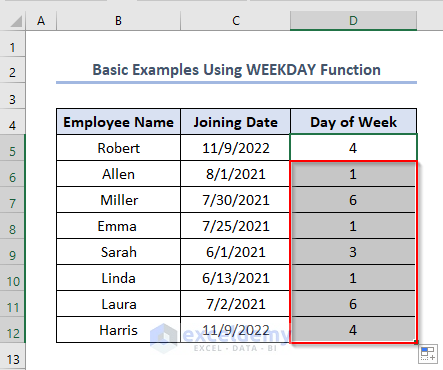
If the days are given in date format and do not need a return_type value, you may utilize the following formula in the D5 cell.
=WEEKDAY(C5)Here, C5 is the Joining Date of Robert.
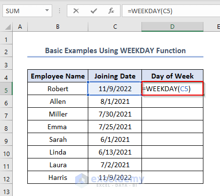
- Press ENTER.
- Use the Fill Handle by dragging down the cursor while holding it at the right-bottom corner of the D5 cell like this.
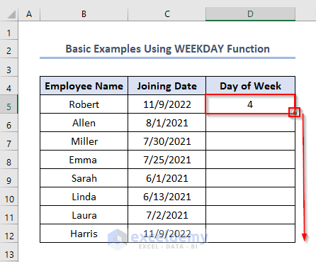
- The outputs will look like this.
But if the return_type is 2 and 16 respectively for the same dataset, you may use the following formula in the D5 cell.
- When the value of return_type is 2:
=WEEKDAY(C5,2)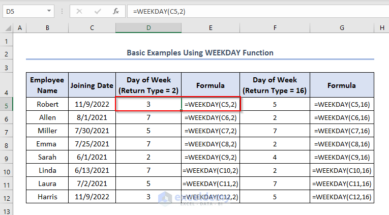
- When the value of return_type is 16:
=WEEKDAY(C5,16)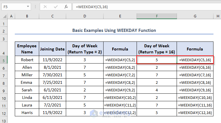
Example 2 – Using WEEKDAY Function with DATE Function
If joining date is given in serial number, you have to use the DATE where the YEAR, MONTH, and DAY functions to return the year, month, and day of the given date respectively.
- Enter the following formula in D5
=WEEKDAY(DATE(YEAR(C5),MONTH(C5),DAY(C5)),12)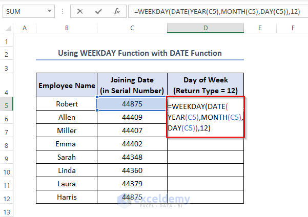
- Press ENTER.
- Use the Fill Handle.
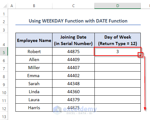
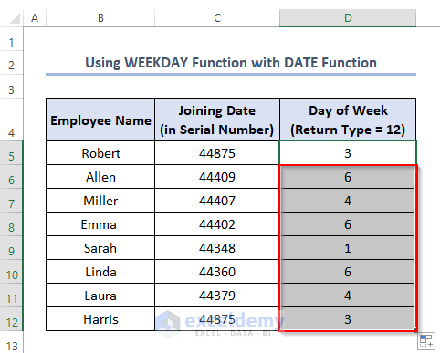
- The following output is returned.
Example 3 – Using TEXT Function to Find Weekday Name
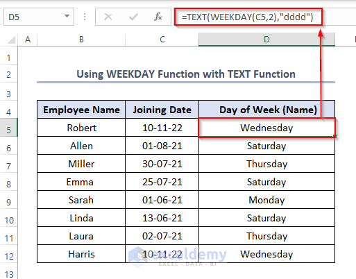
If you want to get the name of the day of the week that is found using the WEEKDAY function, you may use the TEXT function.
- Enter the below formula in the D5 cell.
=TEXT(WEEKDAY(C5,2),"dddd")- Hit ENTER and then use the Fill Handle to return the results.
Example 4 – WEEKDAY Combined with CHOOSE Function
- Enter the following formula in the D5 cell and then use the Fill Handle to get all the outputs.
=CHOOSE(WEEKDAY(C5),"Sun","Mon","Tue","Wed","Thu","Fri","Sat")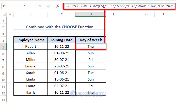
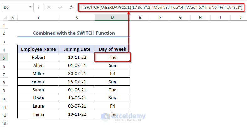
Example 5 – Combined with SWITCH Function
- Enter the below formula in the D5 cell.
=SWITCH(WEEKDAY(C5,1),1,"Sun",2,"Mon",3,"Tue",4,"Wed",5,"Thu",6,"Fri",7,"Sat")
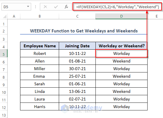
Example 6 – WEEKDAY Function to Get Weekdays and Weekends
Apply the following formula in cell D5.
=IF(WEEKDAY(C5,2)<6,"Workday","Weekend")
Example 7 – WEEKDAY Function with Conditional Formatting
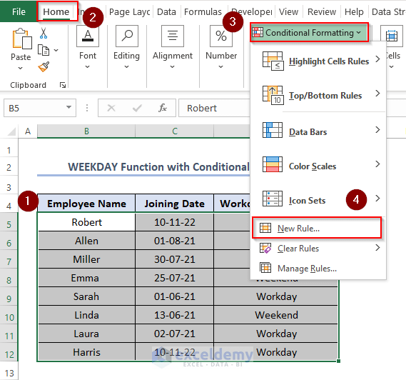
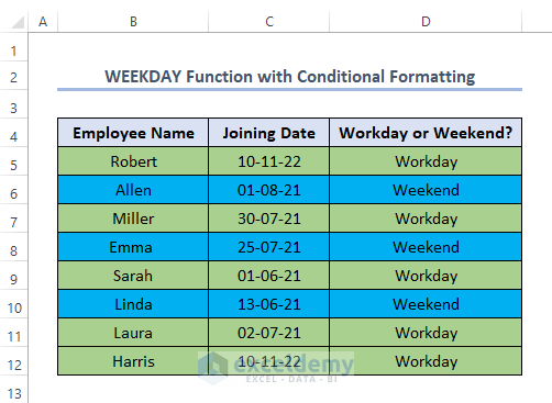
If you need to highlight the workday and weekend for better visualization, you may use the Conditional Formatting toolbar from the Styles command bar.
Steps:
- Select the cells B5:D12.
- Go to Home > choose Conditional Formatting > select New Rule.
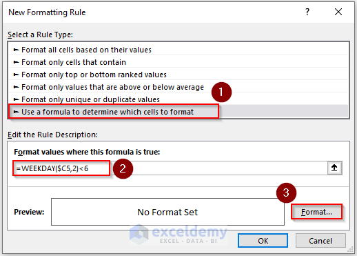
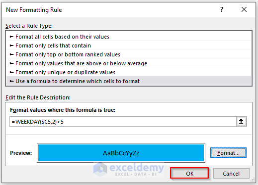
- A New Formatting Rule window will appear.
- Choose Use a formula to determine which cells to format.
- Enter the below formula in the formula box.
=WEEKDAY($C5,2)<6- Go to Format to select the color of the output.
- Click OK.
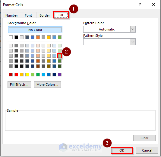
- In the New Formatting Rule, click OK.
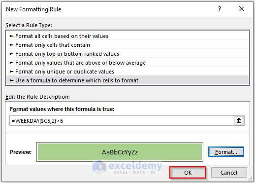
- Go to New Formatting Rule after selecting the cells. Enter the following formula.
=WEEKDAY($C5,2)>5- Go to Format.
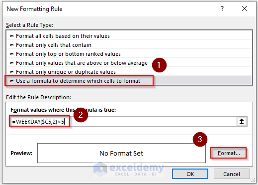
- Select any color in the Fill option, here the light blue color is selected.
- Click OK.
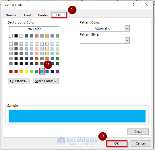
- Click OK in the New Formatting Rule
- The outputs will look like this.
Example 8 – Calculating Payment Including Weekends
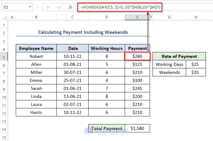
In the sample dataset the number of working hours is given and you need to calculate the Payment for each employee and the total payment for all employees.
The formula will be entered in the E5 cell.
=IF(WEEKDAY(C5, 2)>5, D5*$H$6,D5*$H$7)Use the SUM function for aggregating the individual payment.
Excel WORKDAY Function for Holidays
Excel’s WORKDAY function can be used to determine the work date that will occur a certain number of days after the start date.
The syntax of the WORKDAY function is.
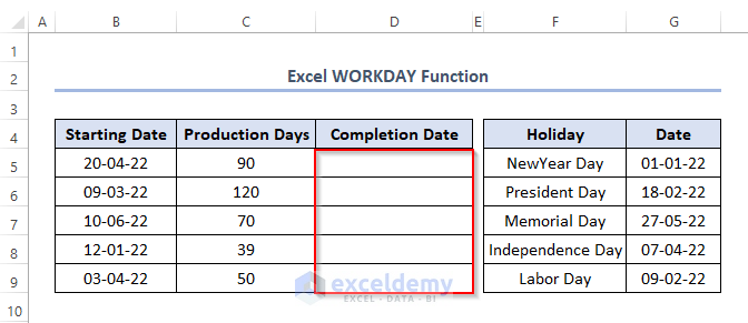
The sample dataset has column headers for Starting Date, Production Days, and Completion Days.
It also has columns for Holidays and their corresponding Date.
In the Starting Date column are project start dates, in Column C there is the estimated time needed to complete those projects.
We need to return the Completion Date in Column D.
- Enter the following formula in the D5 cell.
=WORKDAY(B5,C5,G5:G9)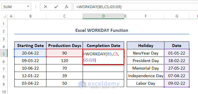
- Press ENTER
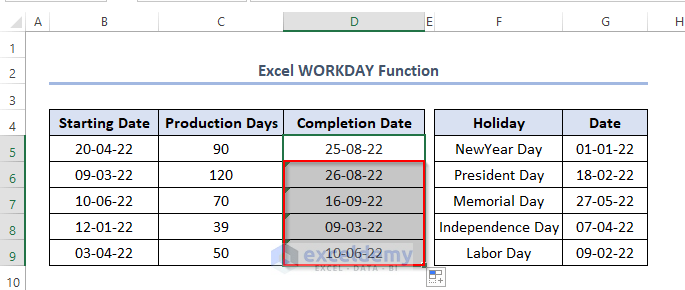
- Use the Fill Handle.
- The outputs of project Completion Dates are returned.
Common Errors While Using WEEKDAY Function
- #NUM – if the serial number is out of range for the current date’s base value – if the return_type is out of range from the return_type value table as shown in the arguments section.
- #VALUE! – occurs when either the given serial_number or the given [return_type] is non-numeric.
Download Excel Workbook
<< Go Back to Excel Functions | Learn Excel
Get FREE Advanced Excel Exercises with Solutions!

