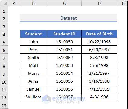
How to Extract Month and Day from a Date in Excel

This dataset showcases Students and their Date of Birth.

Method 1 – Using the Format Cells Option

Steps:

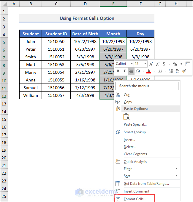
Select the entire range containing dates.
Right-click the column and select Format Cells.

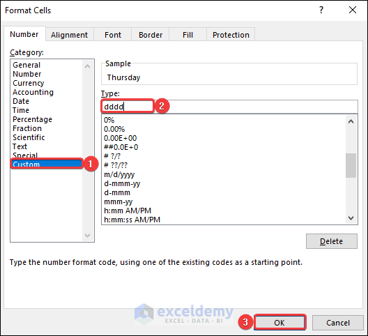
In Format Cells, select Category and choose Custom.
In Type, enter mmmm.
Click OK.

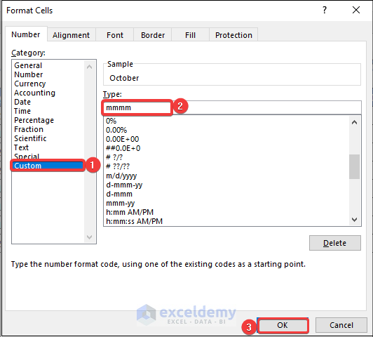
Note: You can also press CTRL + 1 to open the Format Cells dialog box.

The month is extracted from the date.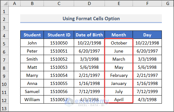

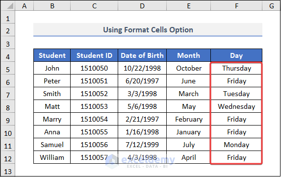
Repeat the same procedure for the Day column.
In Type, enter dddd.
Click OK.

Day is extracted from the date.

Method 2 – Applying the TEXT Function

Steps:

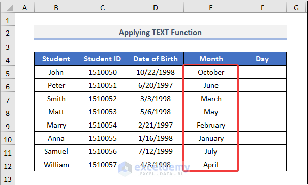
Go to E5 and enter the formula.

=TEXT(D5,”mmmm”)

‘=TEXT’ selects D5. “mmmm” shows the month.

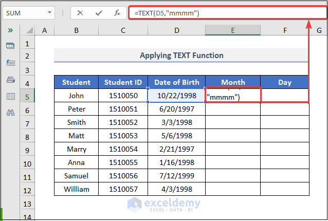
Press ENTER and drag down the Fill Handle to fill E5:E12.

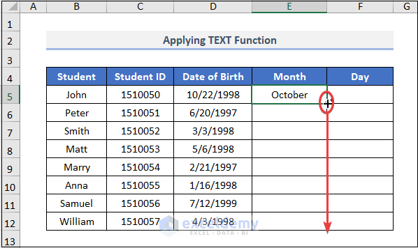
This is the output.

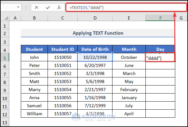
Select F5 and enter the formula.

=TEXT(D5, “dddd”)

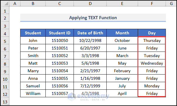
‘=TEXT’ selects D5. “dddd” shows the month.

This is the output.

Method 3 – Using the MONTH and DAY Functions

Steps:

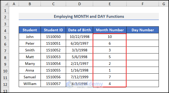
Inl E5, insert the formula.

=MONTH(D5)

It takes the date as input and returns the Month Number of D5.

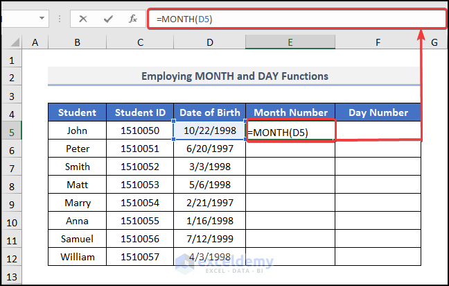
Press ENTER and drag down the Fill Handle.

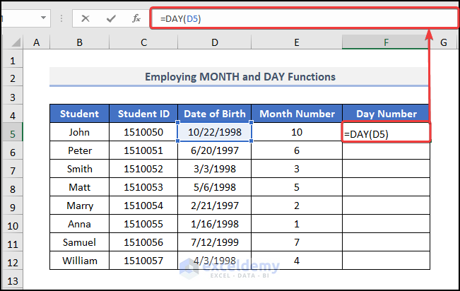
Enter the formula in F5.

=DAY(D5)

The DAY(D5) syntax takes the date in D5 and returns the Day Number.

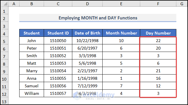
This is the output.

Method 4 – Using the Power Query Feature

Steps:

Select the entire range and go to the Data tab >> choose From Table/Range under Get and Transform Data.

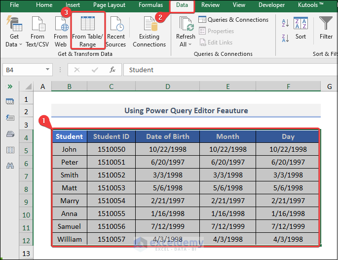
The Create Table dialog box opens. Check My table has headers.

The Power Query Editor will be displayed.

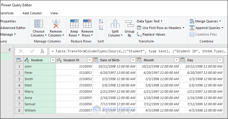
Right-click the Month column and select Transform >> choose Month >> select Name of Month.

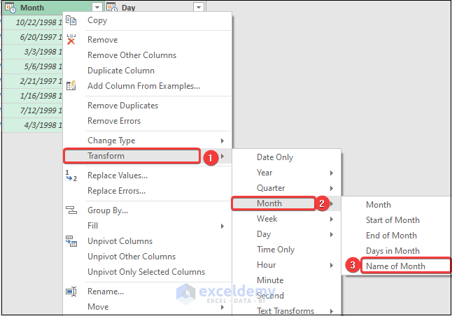
This is the output.

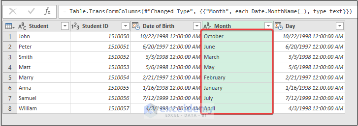
Select the Day column >> choose Transform >> select Day >> click Name of Day.

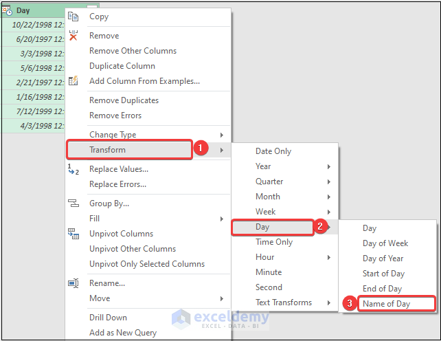
This is the output.

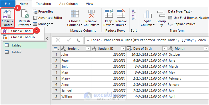
Click Close & Load to see the table in your worksheet.

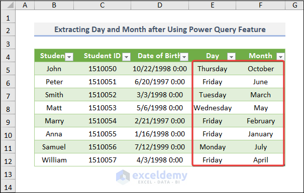
This is the output, after formatting the table.

Method 5 – Using the CHOOSE Function

Go to E5 and enter the formula.

=CHOOSE(MONTH(D5),”Jan”,”Feb”,”Mar”,”Apr”,”May”,”Jun”,”Jul”,”Aug”,”Sep”,”Oct”,”Nov”,”Dec”)

The MONTH function takes the month number from a date. Include the MONTH function in the CHOOSE function and enter the short for month names sequentially. The CHOOSE function selects the month in D5.

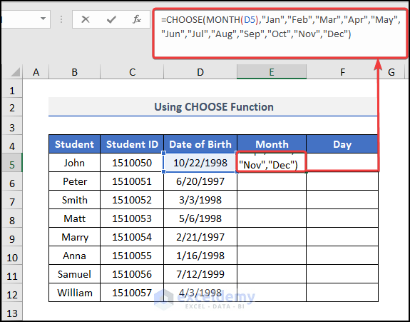
Press ENTER to see the result.

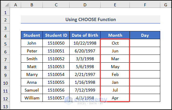
In F5 , enter the formula.

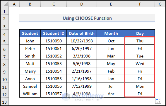
=CHOOSE(WEEKDAY(D5),” Sun”, “Mon”, “Tue”, “Wed”, “Thu”, “Fri”, “Sat”)

The WEEKDAY(D5) syntax takes the number of days from the date, and the CHOOSE function chooses the match for the date.

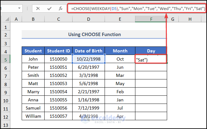
This is the output.

Method 6 – Applying the SWITCH Function

Steps:

Go to E5 and enter the formula.

=SWITCH(MONTH(D5),1,”Jan”,2,”Feb”,3,”Mar”,4,”Apr”,5,”May”,6,”Jun”,7,”Jul”,8,”Aug”,9,”Sep”,10,”Oct”,11,”Nov”,12,”Dec”)

The MONTH function takes the number of months from the date; numbers are the expression_value. The SWITCH function swaps the short for the month name.

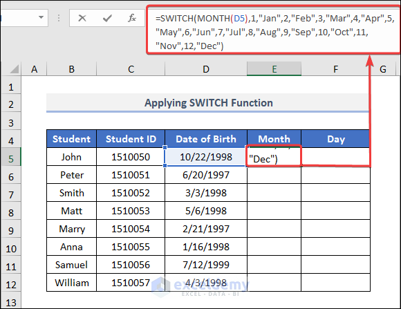
This is the output.

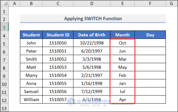
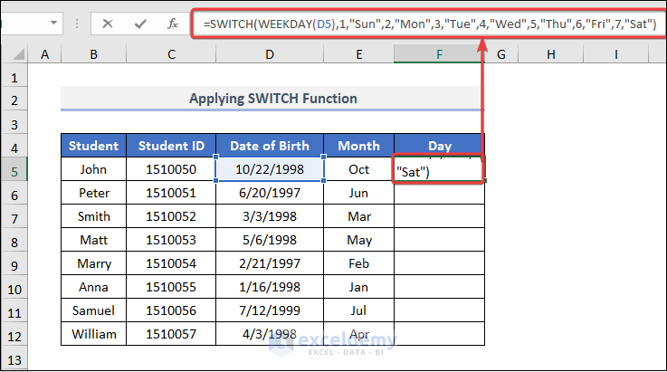
To get the days from the date insert the formula in F5.

=SWITCH(WEEKDAY(D5),1,”Sun”,2,”Mon”,3,”Tue”,4,”Wed”,5,”Thu”,6,”Fri”,7,”Sat”)

Press ENTER and drag down the Fill Handle.

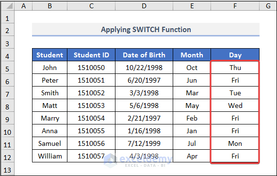
This is the output.

How to Extract Month and Year from Date in Excel

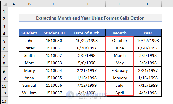
You can extract month and year from the date by using the Format Cells option (extract the month).

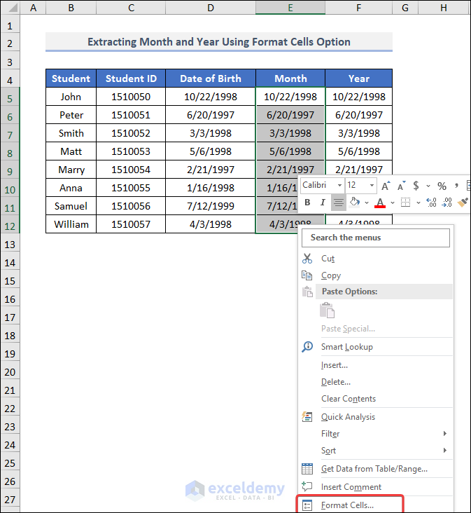
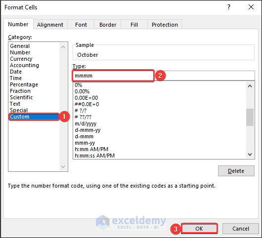
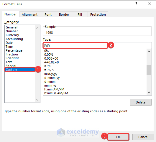
To extract the year, select the entire Date column and press CTRL + 1 to open Format Cells. Choose Custom as Category. Create yyyy in the Type box and click OK.

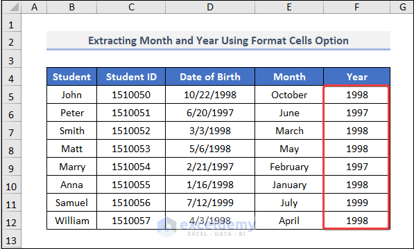
This is the output.

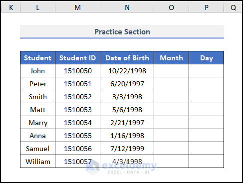
Practice Section

Practice here.

Download Practice Workbook

Download the practice workbook.

Extracting Month and Day from Date.xlsx

<< Go Back To Extract Data Excel | Learn Excel

Get FREE Advanced Excel Exercises with Solutions!

4 Comments

Nicol P. Tyler Nov 16, 2022 at 3:51 PM

Hello Mr. Fahim, I have a dataset of two columns of date. Now, I want find out the numbers of days between these days. Can it be possible? Please help me on it if possible.
- Reply
  Fahim Shahriyar Dipto Nov 17, 2022 at 10:08 AM
  
  Hello Nicol,
  Here’s the solution. You can subtract two dates and can find out the days remaining in your hand. I have attached the step-by-step procedure for better understanding.
  Firstly, go to cell E5 and insert the formula.
  =C5-D5
  
  Secondly, press ENTER and drag down the Fill Handle tool.
  
  Finally, you will get the result like the image below.
Nancy Cruz May 31, 2024 at 2:05 AM

Hello – I have been trying to change a date, 06/23/23 to read 06/23 with no year. When I do it thru the format cells options, it comes back 6/23 – I truly need to sort the column to sort by date and with the zero infront of the 6 it doesn’t sort properly – example: 06/01, 06/02, 06/0
- Reply
  Lutfor Rahman Shimanto Jun 2, 2024 at 9:55 AM
  Hello Nancy Cruz
  
  Thanks for visiting our blog! And also sharing your problem with such clarity. I have reviewed your issue with date formatting and come up with a solution. Please check the following:
  
  Follow these steps:
  1. Select column A and go to Home.
  2. Under the Cells group, expand Format and click on Format Cells.
    // As a result, the Format Cells window will open up.
  3. In the Format Cells window,
    
    Go to Number and click on Custom.
    
    Insert the following formatting code in the Type section: mm/dd
    
    Hit OK.
    // As a result, the date will be formatted as expected like the following:
  4. Now, select the intended date range and apply the desired sorting option.
  Hopefully, you have found the solution you were looking for. I have attached the solution workbook as well. Good luck.
  
  DOWNLOAD SOLUTION WORKBOOK
  
  Regards
  Lutfor Rahman Shimanto
  ExcelDemy