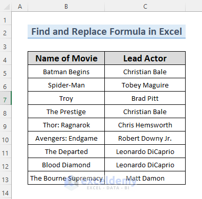
How to Find and Replace Using a Formula in Excel

This is the dataset.

Example 1 – Using Excel FIND and REPLACE Functions

Steps:

Create a new column (Actor’s Short Name, here) and enter the following formula in D5.

=REPLACE(C5,1,FIND(" ",C5),LEFT(C5,1)&". ")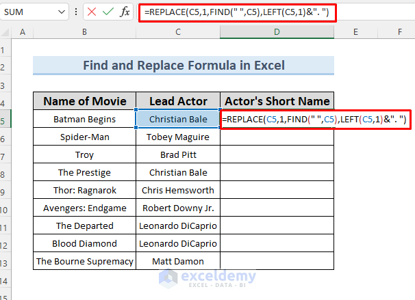

The REPLACE function takes C5 as a reference, counts data until the FIND function finds a space. The LEFT function replaces the first name with its starting alphabet letter followed by a dot (.)

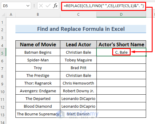
Press ENTER. You will see the output in D5.

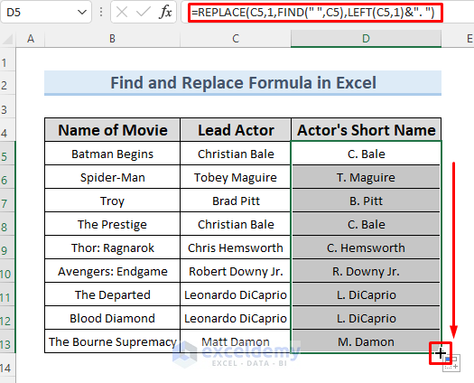
Drag the Fill Handle to AutoFill the other cells.

Example 2 – Using the SUBSTITUTE Function to Find and Replace in Excel

Steps:

Create a new column (Actor’s Short Name, here) and enter the following formula in D5.

=SUBSTITUTE(C5,C5,LEFT(C5,1)&". ") &RIGHT(C5,LEN(C5)-FIND(" ",C5))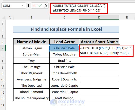

Formula Breakdown

The nested LEFT, RIGHT, LEN, and FIND functions were used in the SUBSTITUTE function to replace the first name of the lead actors with their corresponding first alphabet.

LEN(C5) —-> Returns the number of characters in C5.
- Output: 14
FIND(” “,C5) —-> Returns the position of the space in C5.
- Output: 10
RIGHT(C5,LEN(C5)-FIND(” “,C5)) —-> becomes
RIGHT(C5,14-10) —-> turns into
RIGHT(C5,4)
- Output: Bale
LEFT(C5,1)&”. ” —-> becomes
C & “.”
- Output: C.
SUBSTITUTE(C5,C5,LEFT(C5,1)&”. “) &RIGHT(C5,LEN(C5)-FIND(” “,C5)) —-> Reduced to
SUBSTITUTE(C5,C5, “C. Bale”)
- Output: C. Bale

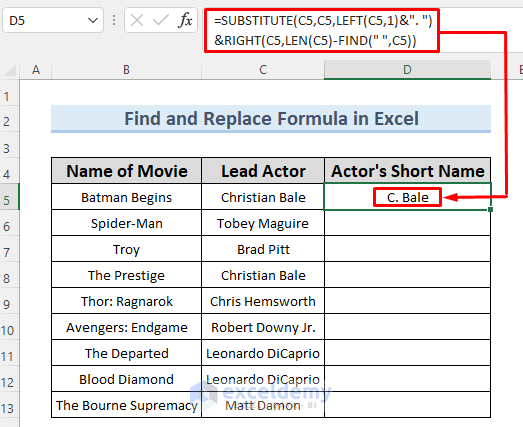
The first name in C5 is replaced with the first alphabet letter followed by a dot.

Press ENTER to see the output in D5.

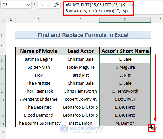
Drag the Fill Handle to AutoFill the other cells.

Example 3 – Find and Replace Cells Using the Excel XLOOKUP Function

Steps:

The dataset was changed. New columns were created (Name of Movie and Full Name of movie, here)

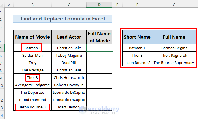
Enter the following formula in D5.

=XLOOKUP(B5,$F$5:$F$7,$G$5:$G$7,B5)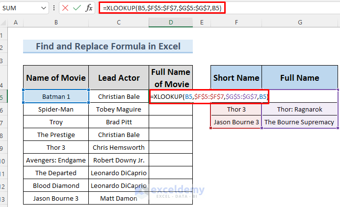

Here, $F$5:$F$7 and $G$5:$G$7 are the lookup_array and the return_array. If the value in B5 matches the lookup_array, then the return_array returns the corresponding value. If he value can’t be found, the cell value will be returned. Value from B5 “Batman 1” is found, therefore, it returns “Batman Begins”.

Press ENTER to see the output in D5.

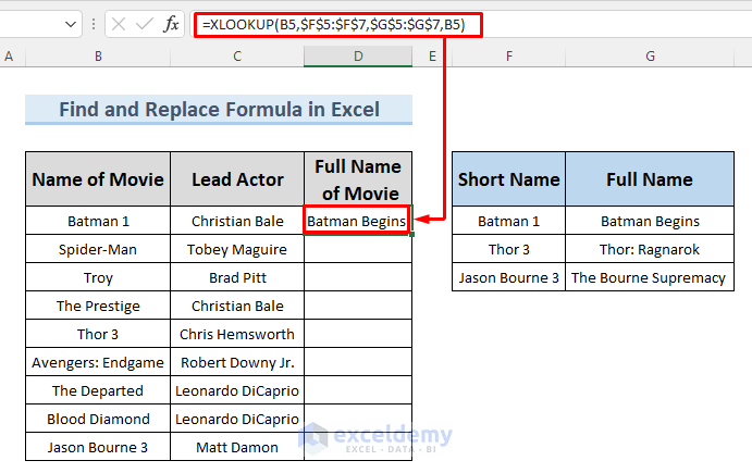
Drag the Fill Handle to AutoFill the other cells.

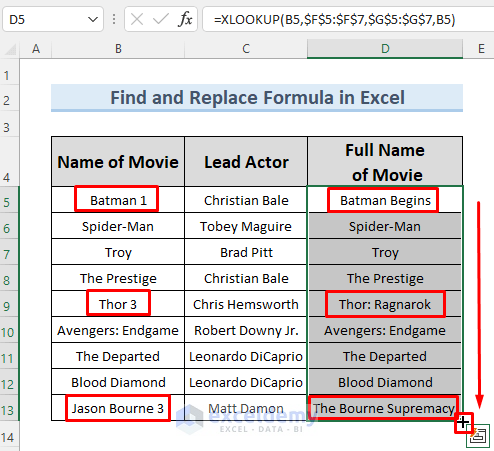
Example 4 – Using the Excel VLOOKUP Function to Find and Replace

Steps:

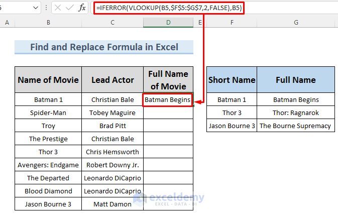
The dataset was changed (movie names were altered and a new column was created).

Enter this formula in D5.

=IFERROR(VLOOKUP(B5,$F$5:$G$7,2,FALSE),B5)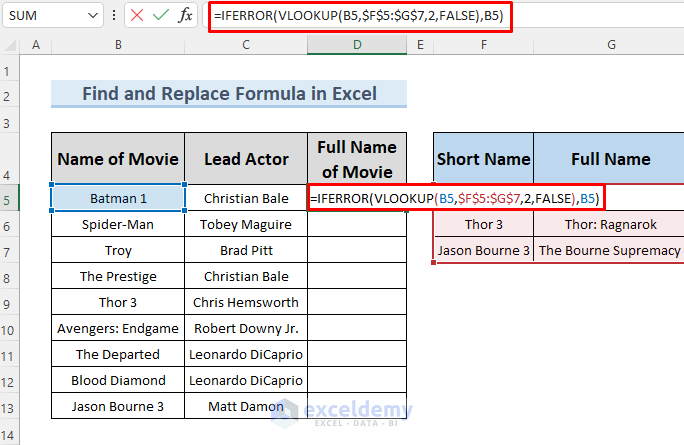

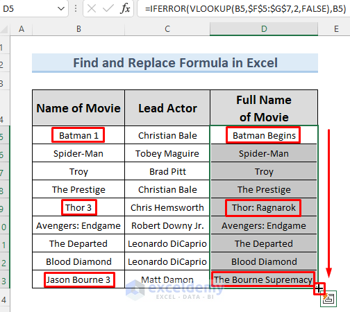
The VLOOKUP function is used to replace words. If a value is not found, it will return an error. The IFERROR function replaces errors with the corresponding cell values. 2 is used in the formula because the output is in the second column of the lookup array. FALSE is used for an exact match.

Note: Use an Absolute Cell Reference.