How to Find Duplicates in Excel Workbook (5 Methods)

Q: How do I find total duplicates in Excel?

The easiest way to count duplicates in Excel is to use COUNTIF(). This function counts the number of cells within the specified range that meets the criteria. For instance, the formula is =COUNTIF( A2:A16, “Monitor”), where Monitor is the criteria.

Q: Can Excel hide duplicates?

Yes, on the Data tab, point to Sort & Filter, and then click Advanced. In the Advanced Filter dialog box, click Filter the list, in place. Select the Unique records only check box, and then click OK. The filtered list is displayed and the duplicate rows are hidden.

Suppose there are two sheets in the workbook named Sheet1 and Sheet2. Sheet1 represents the employee name with their states while Sheet2 displays the joining date along with their name. Here, we have highlighted the duplicate names in Sheet1.

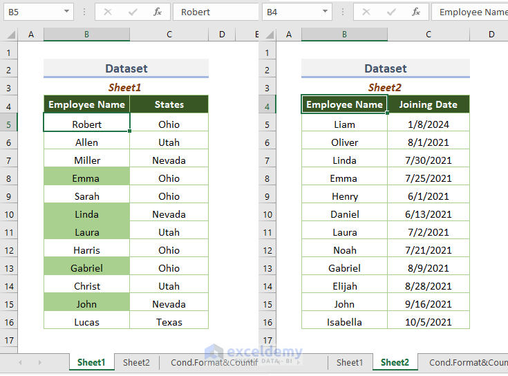
Method 1 – Using Conditional Formatting and the COUNTIF Function

Select the cell range.
Go to the Home tab and the Styles group.
Click on Conditional Formatting and select New Rule.

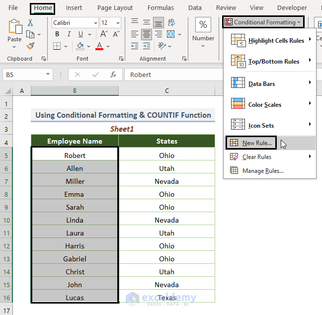
In the New Formatting Rule dialog box, select a Use a formula to determine which cells to format.
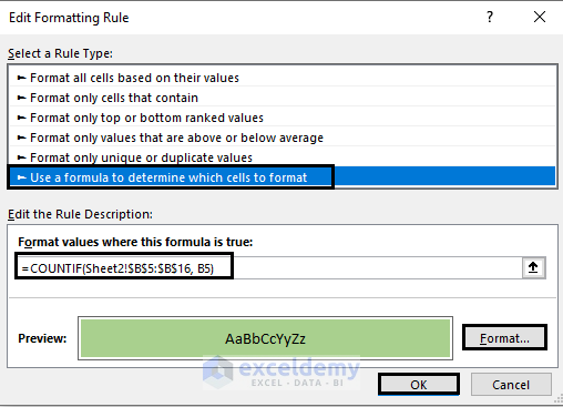
Go to the Edit the Rule Description section.
Insert the formula:=COUNTIF(Sheet2!$B$5:$B$16, B5)
Replace Sheet2 with your second sheet name, $B$5:$B$16 with cell range, and B5 with the first cell.
Open the Format option to specify the highlighting color.
Press OK.

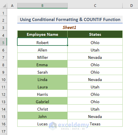
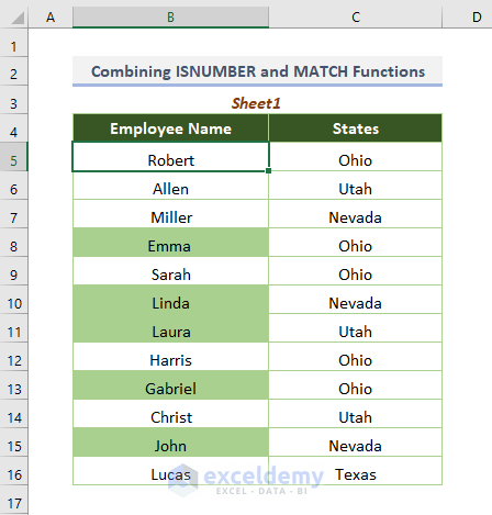
You’ll get the following output. The highlighted names are duplicates also present in Sheet2.

You can also combine the ISNUMBER function with the MATCH function to set up the condition in the Conditional Formatting.

Use this formula in the New Formatting Rule dialog box: =ISNUMBER(MATCH(B5, Sheet2!$B$5:$B$16,0))
Replace Sheet2 with your second sheet name, $B$5:$B$16 with cell range, and B5 with the first cell. The MATCH function returns the relative position of a value in the range and the ISNUMBER function checks if the result of the MATCH function is a number or not.
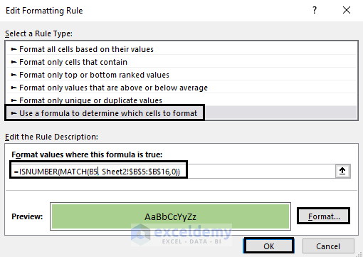
This is the output.

Method 2 – Combining IF and COUNTIF Functions

Select a blank cell in the sheet where you want to find the duplicates.
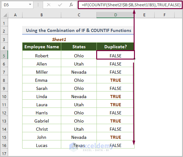
Apply the formula:=IF(COUNTIF(Sheet2!$B:$B,Sheet1!B5),TRUE,FALSE)
Replace Sheet1 and Sheet2 with your sheet names, $B:$B with the column, and B5 with the first cell.
Use the Fill Handle to copy the formula down.
The output TRUE means the corresponding name has duplicate values in Sheet2.

Method 3 – Combining IF, ISERROR, and VLOOKUP Functions

Select an empty cell in the sheet to search for duplicates.
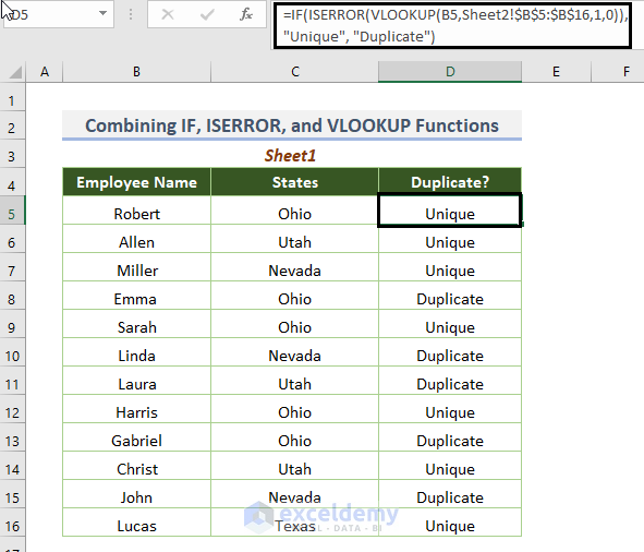
Apply the formula:=IF(ISERROR(VLOOKUP(B5,Sheet2!$B$5:$B$16,1,0)),"Unique", "Duplicate")
Replace Sheet1 with your first sheet name, $B$5:$B$16 with the column, and B5 with the first cell.
The output Duplicate indicates the duplicate values that are present in Sheet1 as well.

Method 4 – Using the EXACT Function

Select a blank cell in the sheet where you need to find duplicates.
Apply the formula:=EXACT(B5,Sheet1!B5)
Replace Sheet1 with your sheet name and B5 with the first cell.
The output TRUE means the corresponding name has exact duplicate values in Sheet1.

Method 5 – Using Excel Power Query

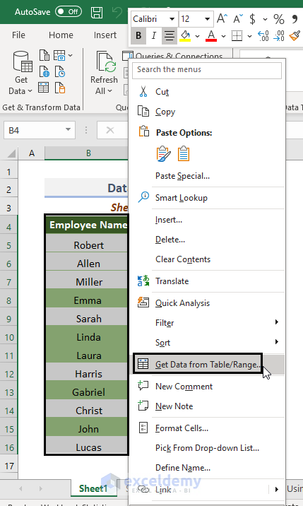
Select the cell range.
Right-click to open the Context Menu.
Select Get Data from Table/Range.

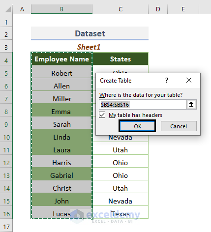
In the Create Table dialog box, click OK.

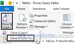
The Power Query Editor window will appear.
Go to the Close & Load drop-down and choose Close & Load To.

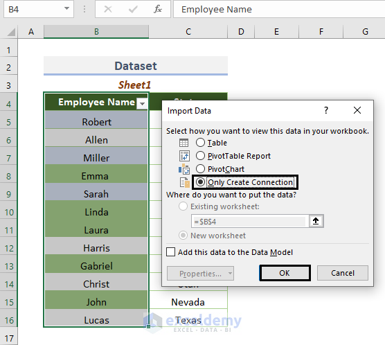
In the Import Data dialog, select Only Create Connection and click OK.

Repeat these steps for the other sheet.
Go to the Data tab and the Get & Transform Data group.
Select Get Data, choose Combine Queries, and click on Merge.

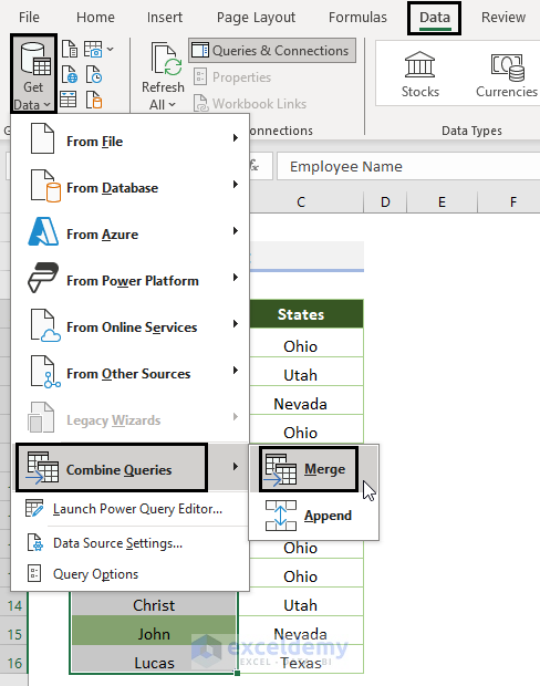
In the Merge window, select the tables and click on the columns.
Select Inner as the Join Kind and click OK.

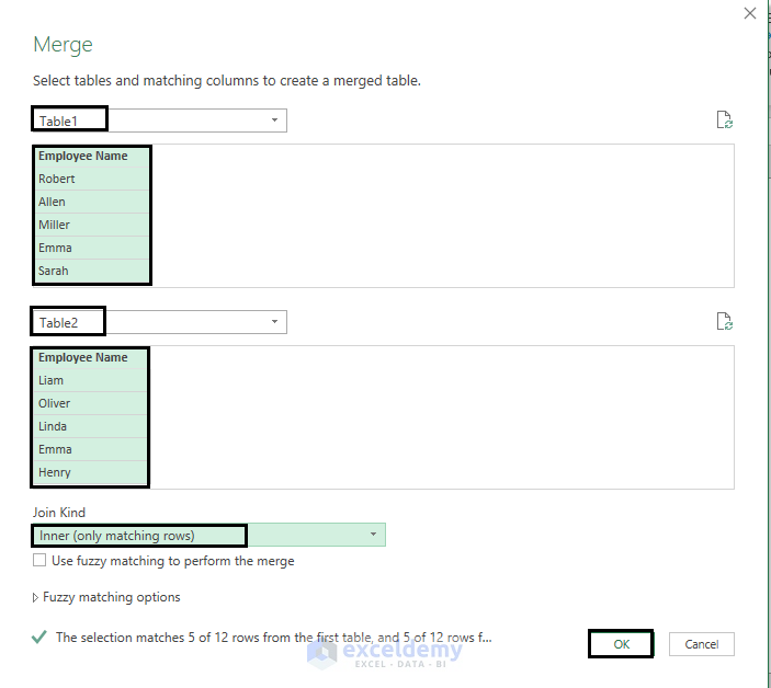
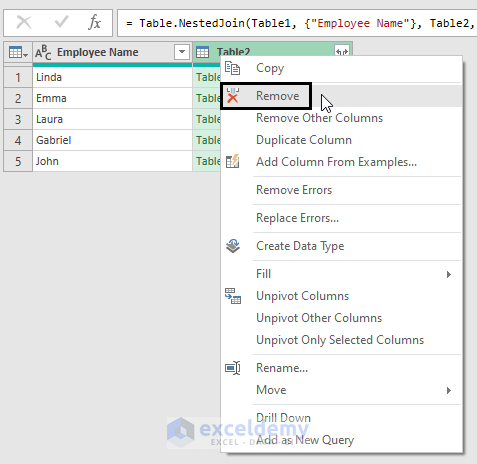
The Power Query Editor window will appear again, containing combined data from the two tables.
Right-click on the second column and choose Remove.
Go to the Home tab and choose Close & Load.

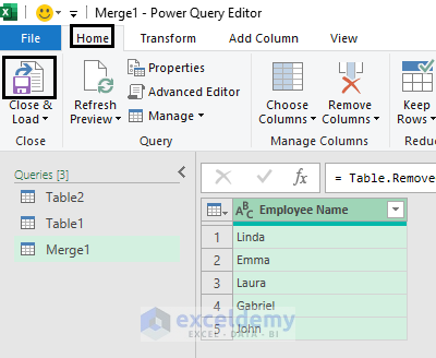
A new worksheet will be created containing only the duplicate values.

Download the Practice Workbook

Find Duplicates in Workbook.xlsx

Frequently Asked Questions

Can Excel automatically find duplicates?

Yes, the fastest way to find and highlight duplicates in Excel is by using Conditional Formatting. The biggest advantage of this method is that it not only shows duplicates in the existing data but automatically checks new data for duplicates right when you enter it in a worksheet.

How do I find total duplicates in Excel?

The easiest way to count duplicates in Excel is to use COUNTIF(). This function counts the number of cells within the specified range that meets the criteria. For instance, the formula is =COUNTIF( A2:A16, “Monitor”), where Monitor is the criteria.

Can Excel hide duplicates?

Yes. On the Data tab, point to Sort & Filter, and then click Advanced. In the Advanced Filter dialog box, click Filter the list, in place. Select the Unique records only check box and click OK. The filtered list is displayed and the duplicate rows are hidden.