How to Find Duplicates in Two Columns in Excel (6 Methods)

Dataset Overview

The below screenshot is an overview the dataset & an example of the function to find duplicate values:

Method 1 – Finding Duplicates within Similar Rows in Two Columns

1.1 Using the Equal Sign as Logical Argument

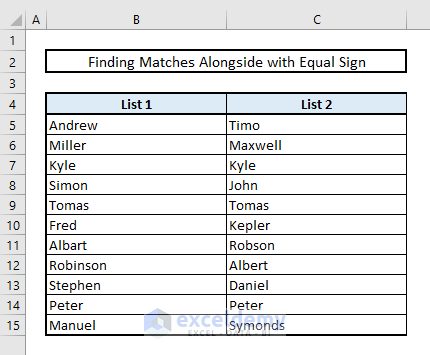
We have two lists of names in Columns B and C.

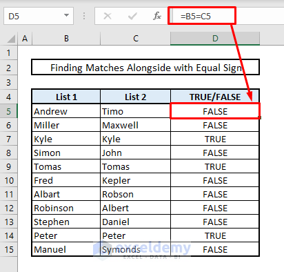
To find duplicates within the same row, use the equal sign as a logical function.

• In Cell D5, enter:

• Press Enter. If matches are found, the value will return as TRUE; otherwise, it will return as FALSE.
• Autofill the rest of the cells in Column D to find all matches.

1.2 Using IF Function

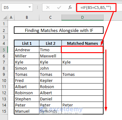
• In Cell D5, enter the following formula:

• Press Enter.
• Autofill other cells in Column D.

Read More: Excel Formula to Find Duplicates in One Column

1.3 Applying Conditional Formatting 

To highlight duplicates within the same rows in two columns:

• Select the range of cells.

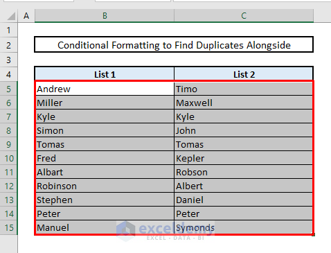
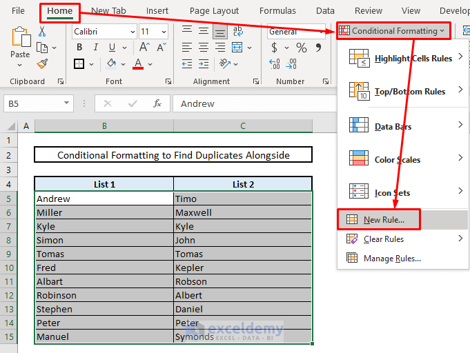
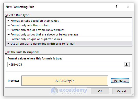
• Under the Home tab, choose Conditional Formatting > New Rule.

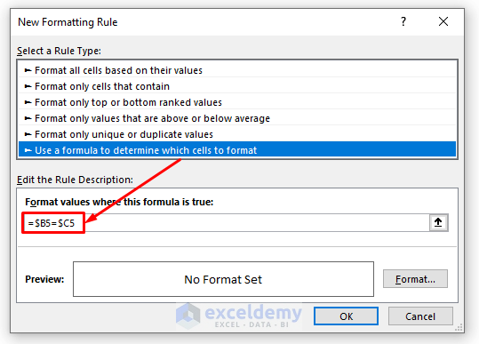
• Use a formula to determine formatting:

 =$B5=$C5

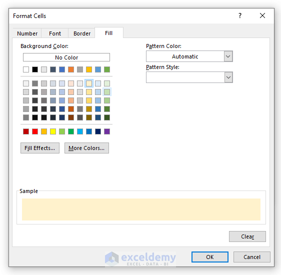
• Select a color for highlighting.

• Confirm to apply the formatting.

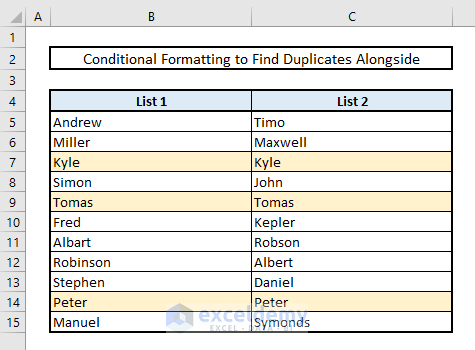
In the picture below, the matches in the same rows are now visible with the selected color.

Read More: How to Find Duplicates in Excel Workbook

Method 2 – Finding Duplicates within Any Rows in Two Columns

2.1 Applying Conditional Formatting

To find duplicates in any rows of two columns:

• Select the range of cells.

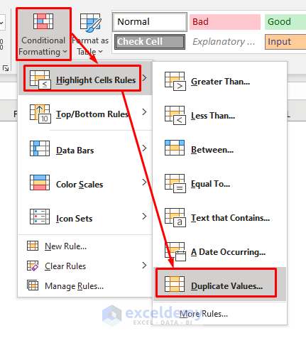
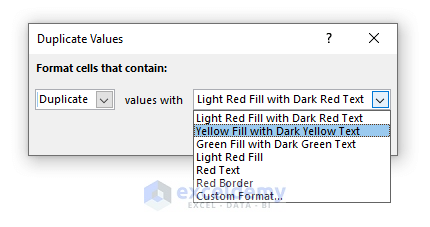
• Under the Home tab, choose Conditional Formatting > Duplicate Values.

• Select a color for highlighting
• Press OK.

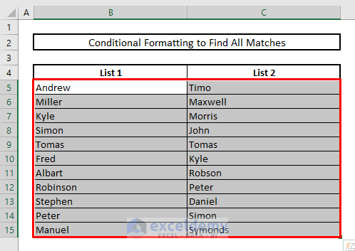
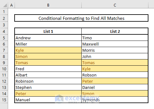
In the picture below, you’ll see all the matches with the highlighted colors.

Read More: How to Find Similar Text in Two Columns in Excel

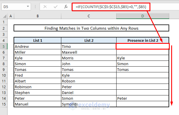
2.2 Combining IF & COUNTIF Functions to Detect Duplicates in Two Columns

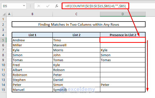
• In Cell D5, enter this formula:

• Press Enter and autofill the rest of the cells in Column D.

Read More: How to Find Duplicate Values Using VLOOKUP in Excel

2.3 Using IF, AND, COUNTIF Functions

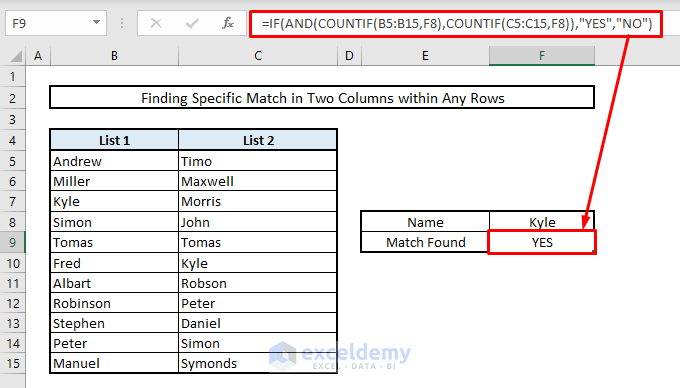
• To check if a specific name is present in both Columns B and C:
  • In Cell F8, enter the name (Kyle).
  • In Cell F9, enter this formula:

• Press Enter. If it shows YES, the name is present in both columns.

Read More: How to Find Duplicates in Two Different Excel Workbooks

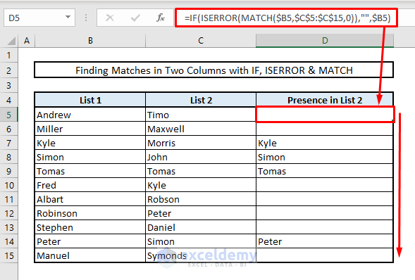
2.4 Combining IF, ISERROR. MATCH Functions

To find matches using the MATCH function:

• In Cell D5, enter this formula:

• Press Enter.
• Autofill the entire column by using Fill Handle.

Method 3 – Finding Duplicates in More Than Two Columns

3.1 Using IF-AND Functions 

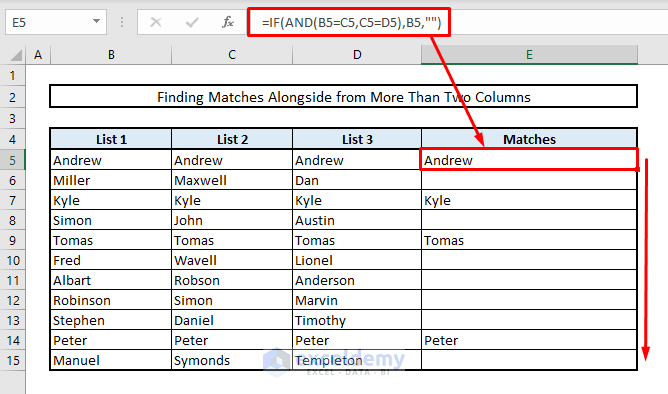
To identify matches or duplicates across more than two columns, we’ll employ the AND function to combine multiple criteria. In our modified dataset, we’ve introduced an additional column (List 3) with additional names. Let’s find all the matches within the same rows in Column E.

• In Cell E5, enter the following formula:

• Press Enter and then autofill the remaining cells in Column E using the Fill Handle. This will display all the matches within the same rows.

3.2 Using IF-OR Functions to Find Duplicates within Similar Rows in Any Two of Multiple Columns

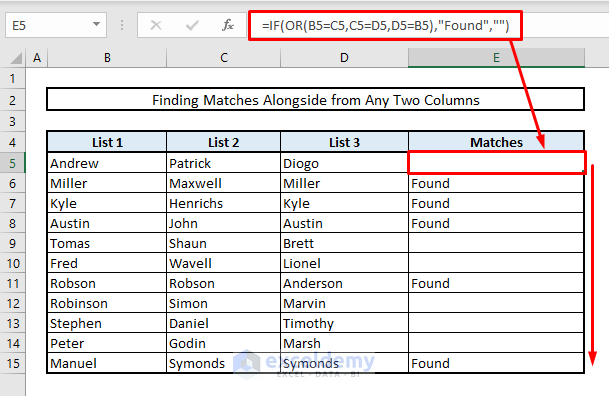
Consider another scenario: finding duplicates within the same rows across any two columns from a set of more than two columns. If matches are found, the message will display Found; otherwise, it will remain blank.

• Press Enter and autofill the remaining cells in the column. This will highlight all the matches found within the same rows.

Read More: How to Find Duplicates without Deleting in Excel

Method 4 – Extracting Data Based on Duplicates in Two Columns

4.1 Using VLOOKUP or INDEX-MATCH

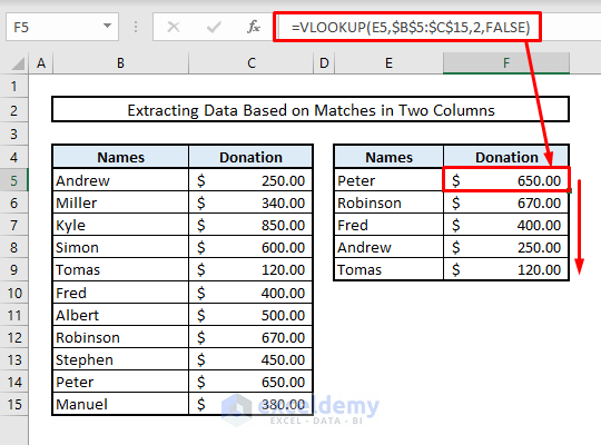
Suppose we want to extract data based on the duplicates found in two columns. In our modified dataset, Columns B and C represent names of individuals along with their corresponding donation amounts. Column E contains a subset of names, and we’ll find the donation amounts for these individuals in Column F by identifying duplicates between Columns B and E.

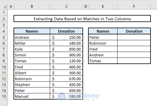
• In Cell F5, enter the following VLOOKUP formula:

• Press Enter and autofill the entire Column F. This will provide the donation amounts for the selected individuals from Column E.

Alternatively, you can achieve similar results using the INDEX-MATCH formula. In this case, the formula in Cell F5 would be:

Then press Enter and autofill the entire column.

4.2 Inserting Wildcard Characters inside VLOOKUP or INDEX-MATCH Functions

Now, let’s assume we have full names in Column B and abbreviated names in Column E. We want to search for partial matches in Column B and extract the donation amounts for the selected individuals in Column F. To achieve this, we’ll use wildcard characters (specifically, an asterisk *) before and after the cell references from Column E. The asterisk acts as a wildcard, allowing us to search for additional text.

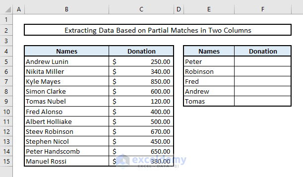
• In Cell F5, enter the following VLOOKUP formula:

• Press Enter and autofill the entire Column F. This will yield the results.

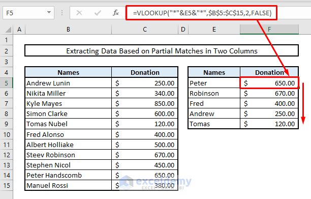
If you prefer to enter INDEX-MATCH functions, enter the following in Cell F5:

Press Enter & use the Fill Handle to fill down the entire column.

Method 5 – Finding Case-Sensitive Duplicates in Two Columns

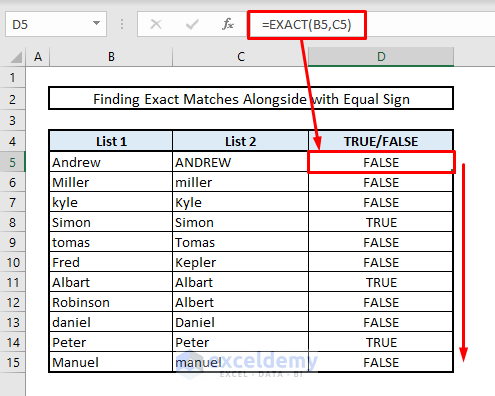
All the methods mentioned above were case-insensitive. If you need to find duplicates in two columns within the same rows while considering case sensitivity, follow this approach. Suppose we have two columns (List 1 and List 2) with some overlapping names, but the case of the letters differs. By using the EXACT function, we can identify which names match exactly, taking case sensitivity into account.

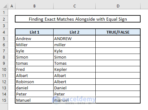
• In Cell D5, enter the following formula:

• Press Enter and autofill the remaining cells using the Fill Down handle. The matches will be shown as TRUE, and any mismatches will return FALSE.

Method 6 – Using VBA Editor to Find Duplicates in Two Columns

Here we are going to show the duplicates in Column D with the help of VBScript.

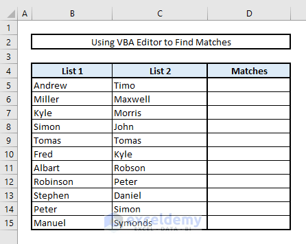
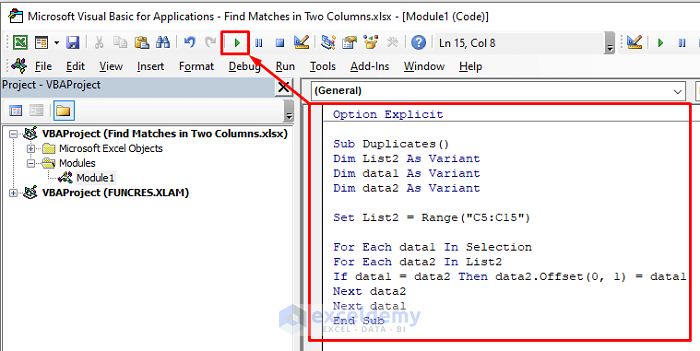
• Press Alt + F11 to open the VBA window.

• From the Insert tab, select Module. This will create a new module in the VBA editor where you can enter your code.

• In the editor window, copy and paste the following code:

Sub Duplicates()
Dim List2 As Variant
Dim data1 As Variant
Dim data2 As Variant
Set List2 = Range("C5:C15")
For Each data1 In Selection
For Each data2 In List2
If data1 = data2 Then data2.Offset(0, 1) = data1
Next data2
Next data1
End Sub

• Click the Run button or press F5 to activate the subroutine.

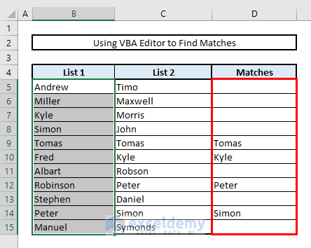
This code will compare the values in the selected range (List 1) with those in Column C (List 2). If a match is found, it will populate the adjacent cell in Column D.

• Close the VBA window by pressing Alt + F11 again to return to your Excel workbook.
• Now select the range of cells from List 1 that you want to inspect for matches in List 2.

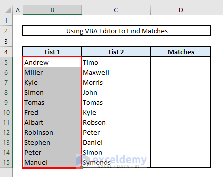
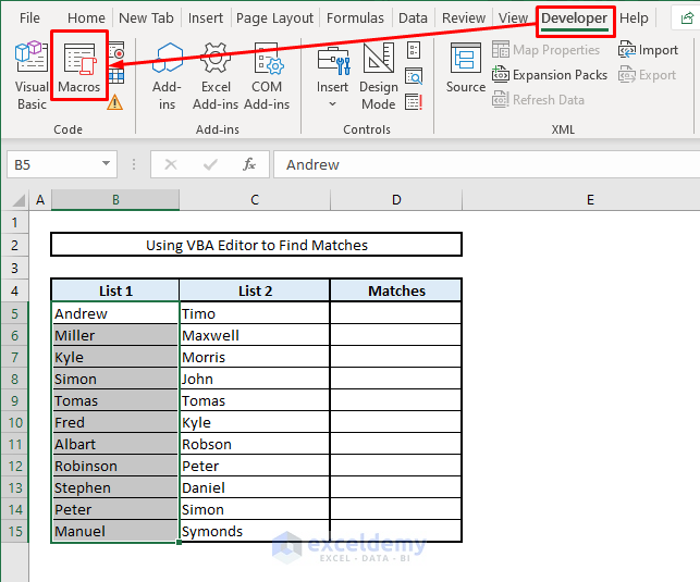
• From the Developer tab (if visible), select Macros. A dialogue box will open.

Note: If you don’t find the Developer option at the top or ribbon section, then you have to enable it by opening Excel Options first. There you’ll find the ‘Customize Ribbon’ option. From the Main Tabs option, put a Select mark on Developer. Press OK & the Developer tab should now appear at the top of your Excel workbook.

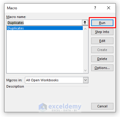
• Choose the macro name (which you’ve already activated) and press Run.

You’ll see all the matches in Column D, as shown in the picture below.

Download Practice Workbook

You can download the practice workbook from here:

<< Go Back to Find Duplicates in Excel Column | Find Duplicates in Excel | Learn Excel