How to Find Duplicates in Two Different Excel Workbooks (5 Methods)

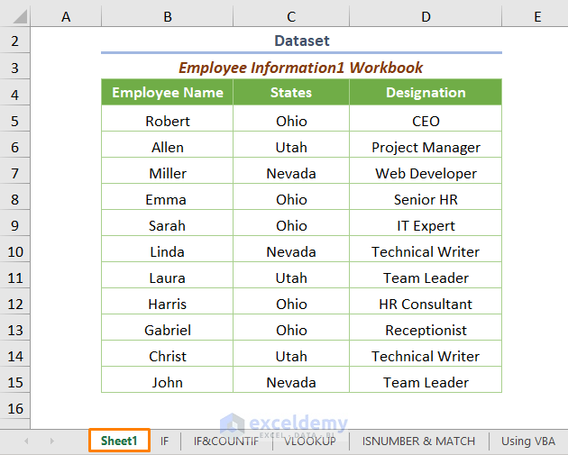
Let’s assume we have two different datasets with a common field (Employee Name) in two different sheets in two workbooks. The first dataset is in Sheet1 of the Employee Information1.xlsm workbook (Workbook1).

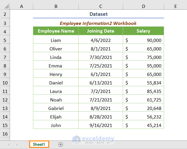
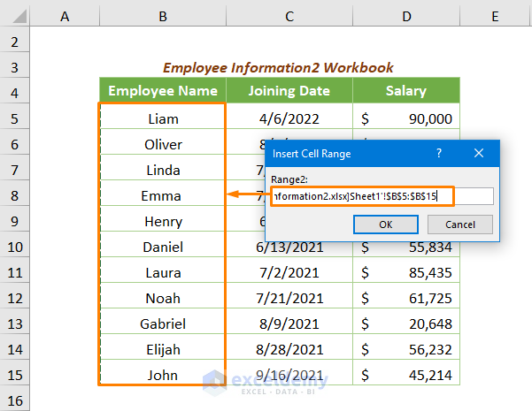
The other one is in Sheet1 of the Employee Information2.xlsx workbook (Workbook2) as shown in the following image.

Let’s learn how to find the duplicates in these two different worksheets.

Method 1 – Using the COUNTIF Function

The COUNTIF function is one of the most popular functions that is used to count the number of cells with given criteria.

While counting duplicates, the generic formula will be like the following.

In the case of finding duplicates in two different workbooks, the adjusted formula will be-

‘[Employee Information2.xlsx]Sheet1’!$B$5:$B$15 is the range where we want to count duplicates. The ‘[Employee Information2.xlsx]Sheet1’ represents the Sheet1 of Workbook2 and B5 is the specific cell that we want to count in cells B5 through B15 at the Workbook2 (criteria).

After inserting the formula, press the ENTER key. You’ll get the following output if you use the Fill Handle Tool.

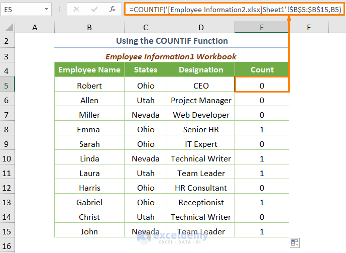
In the above output, you can see that the value of duplicates is 1 and the value of unique records is 0.

Read More: How to Find Duplicate Values Using VLOOKUP in Excel

Method 2 – Using IF and COUNTIF Functions

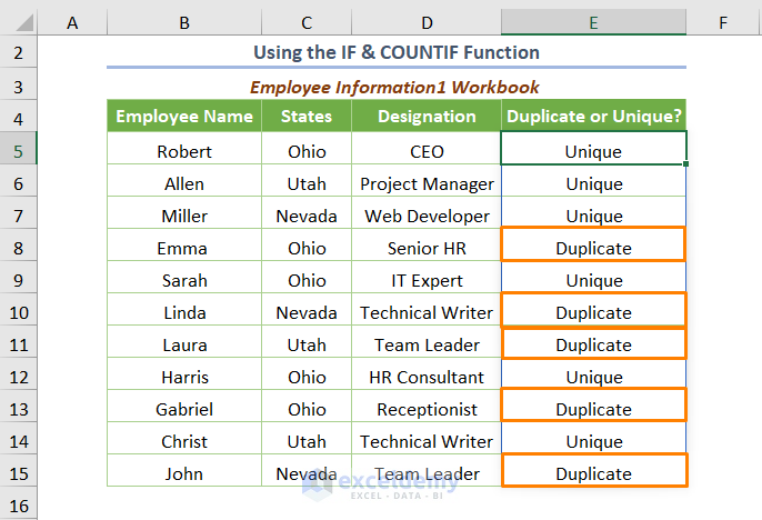
Instead of getting the numerical value, you can find the string “Duplicates” or “Unique”. For this, we can use the following formula.

⧭ If the value of the output using the COUNTIF function is greater than 0, the IF function will return “Duplicates”. Else it’ll return “Unique”.

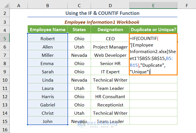
Note: here, we inserted the criteria as a range B5:B15. In such a situation, you don’t need to copy the formula for the remaining cells. You’ll get the output by pressing ENTER.

Read More: How to Find Duplicates without Deleting in Excel

Method 3 – Applying the VLOOKUP Function to Find Duplicates in Two Workbooks

The VLOOKUP function together with the IF and IFERROR function may be used to get the duplicates in two different Excel workbooks.

B5 is the starting cell of Workbook1. 1 is the col_index_num argument and 0 is for approximate match.

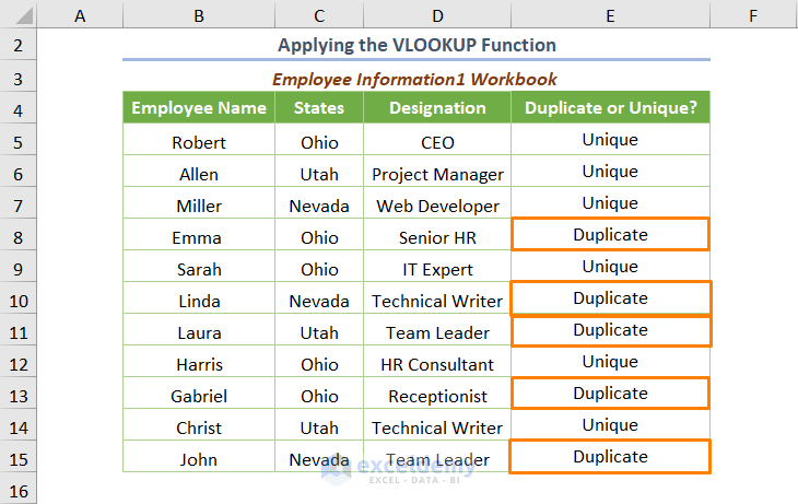
⧭ In the above formula, the VLOOKUP function will return the Employee Name if it finds similar values in Workbook2 (duplicates). Else, it will return the #N/A error. Therefore, the ISERROR function is used to avoid any display of errors. The IF function provides the output as “Duplicates” or “Unique”.

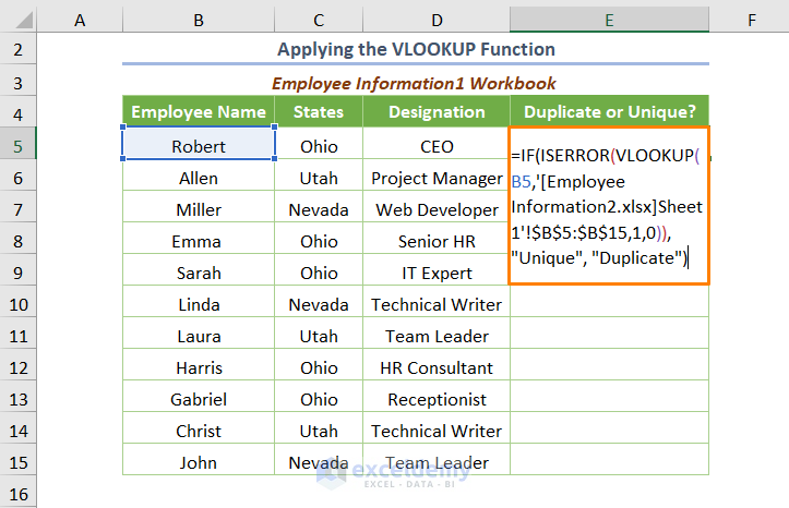
Press ENTER and drag down the formula. You’ll get the following output.

Read More: Excel Formula to Find Duplicates in One Column

Method 4 – Utilizing ISNUMBER and MATCH Functions

The ISNUMBER function combined with the MATCH function can be used to show duplicates. The combined formula is-

⧭ In this formula, the MATCH function finds the relative position in the numeric value e.g. 4 for the B8 cell of the matched lookup value. Otherwise, it will return the #N/A error. The ISNUMBER function is used to display TRUE instead of showing the number and FALSE for the #N/A error.

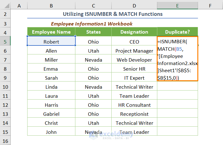
The output will be as follows.

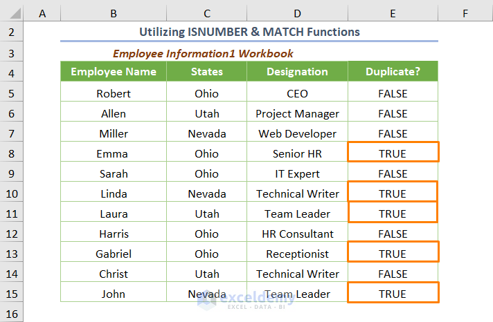
TRUE represents “Duplicates” and FALSE represents “Unique” records.

Read More: Find and Highlight Duplicates in Excel

Method 5 – Using the VBA Code to Find Duplicates in Two Excel Workbooks

VBA code can be used to find the duplicates in two different workbooks as well as highlight the duplicate values.

Open a module by clicking Developer > Visual Basic.

Go to Insert > Module.

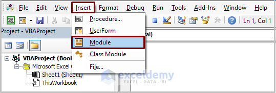
Enter the following code into the newly created module.

Sub Duplicates_Workbooks_VBA()
Dim RngWorkbook1 As Range, RngWorkbook2 As Range, Rn1 As Range, Rn2 As Range
Set RngWorkbook1 = Application.InputBox("Range1:", "Insert Cell Range", Type:=8)
Set RngWorkbook2 = Application.InputBox("Range2:", "Insert Cell Range", Type:=8)
For Each Rn1 In RngWorkbook1
    Rn1Value = Rn1.Value
    For Each Rn2 In RngWorkbook2
        If Rn1Value = Rn2.Value Then
            Rn1.Interior.Color = VBA.RGB(255, 255, 0)
            Exit For
        End If
    Next
Next
End Sub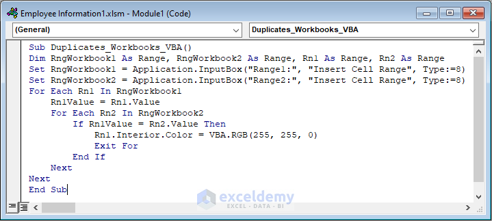

⧭ In the above code, we declared necessary variables. We have used the InputBox to insert the cell range for Workbook1 and Workbook2 respectively. We have used the For loop to find the duplicates in those workbooks. We have assigned the VBA RGB function to highlight the color. Specifically, we have used 255 as the value of the red and green arguments and 0 for the blue argument to highlight duplicates values in yellow color.

Run the code (the keyboard shortcut is F5 or Fn + F5). You’ll get the input box to insert the cell range of Workbook1.

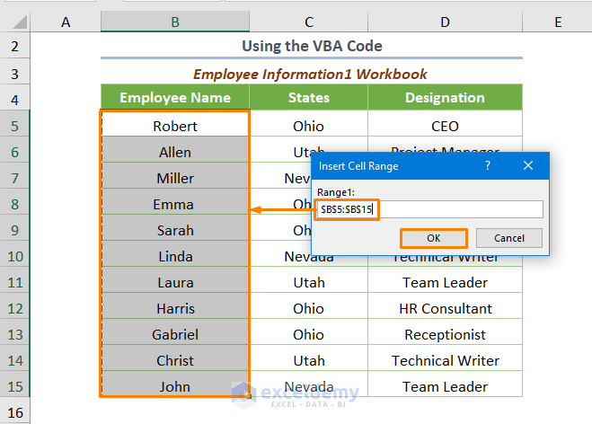
After pressing OK, you’ll get another input box to insert the cell range of Workbook2.

You’ll get the highlighted duplicates values as shown in the following image.

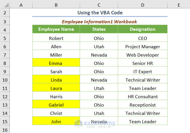
Note: If you want to highlight duplicate values along with two workbooks, this method is recommended because the Conditional Formatting tool doesn’t work for two workbooks. It is handy for highlighting duplicates across multiple sheets in a workbook.

Read More: Find Duplicates in Two Columns in Excel

Download Practice Workbook

Related Articles

• How to Find Similar Text in Two Columns in Excel
• How to Find Duplicates in Excel Workbook

<< Go Back to Find Duplicates in Excel | Learn Excel