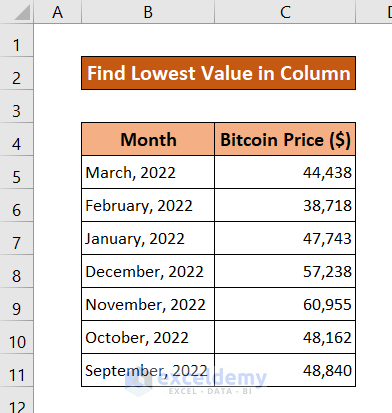
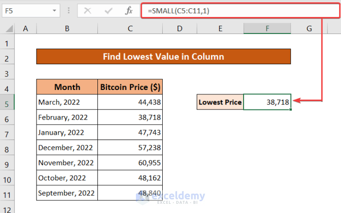
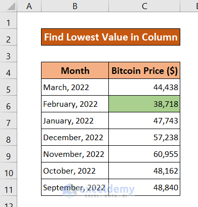
To demonstrate all the methods, we’ll use the same dataset below. It shows Bitcoin prices by months in dollars. We’ll look for the lowest price on the list and show the month with that value.
Method 1 – Find the Lowest Value in a Column Using the AutoSum Feature
Steps:
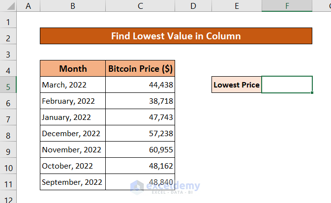
- Select the cell you want your minimum value to be displayed.
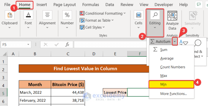
- In the Home tab, go to Editing.
- Go to the ΣAutoSum function and click on the down arrow beside it.
- Select Min from the drop-down list.
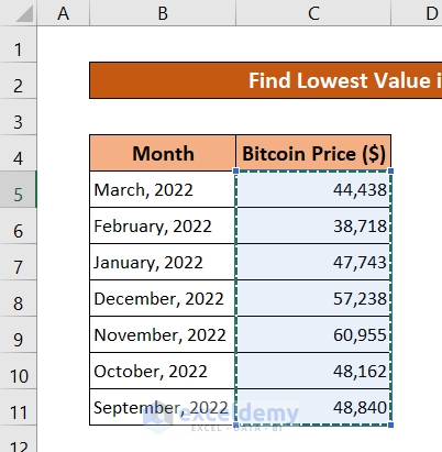
- Select the column you want the minimum value from.
- Press Enter.
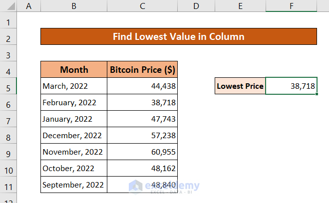
- Excel will put the value into the cell.
Read More: How to Find Highest Value in Excel Column
Method 2 – Using the MIN Function to Find the Lowest Value in a Column
Steps:
- Go to the cell you want your minimum value to be displayed.
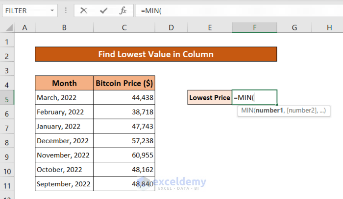
- Use the following formula:
=MIN(C5:C11)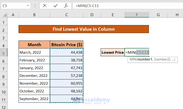
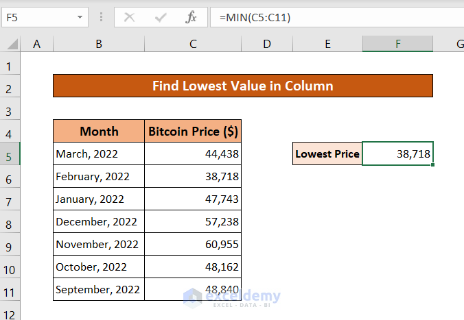
- Press Enter. You will have your lowest value from the column.
Method 3 – SMALL Function to Find the Lowest Value
Steps:
- Go to the cell you want to see your minimum value.
- Insert the following formula. (We use 1 as the second argument to find the smallest value of the array)
=SMALL(C5:C11,1)- Press Enter.
Method 4 – Find the Lowest Value in a Column Using Conditional Formatting
Steps:
- Select the column you want your lowest value from.
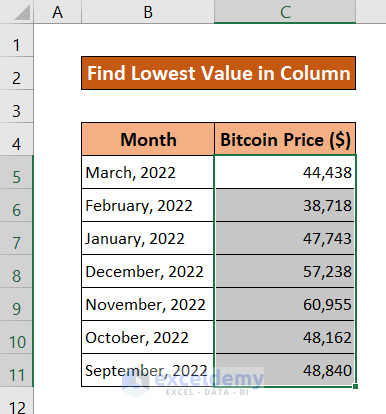
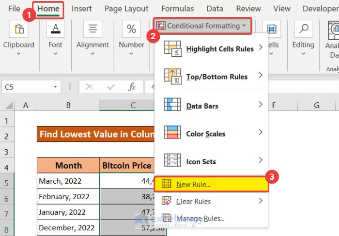
- In the Home tab, under the Styles group, go to Conditional Formatting.
- Select New Rule from the drop-down list.
- A New Formatting Rule box will appear. Under Select a Rule Type, select Use a formula to determine which cells to format.
- In the Format values box, use the following formula.
=C5=MIN(C$5:C$11)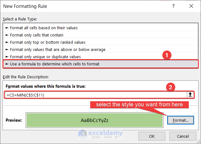
- You can select your cell style from the Format option (we have used Fill Color green here).
- Click on OK.
Method 5 – Using the “Bottom 10 Items” Option
Steps:
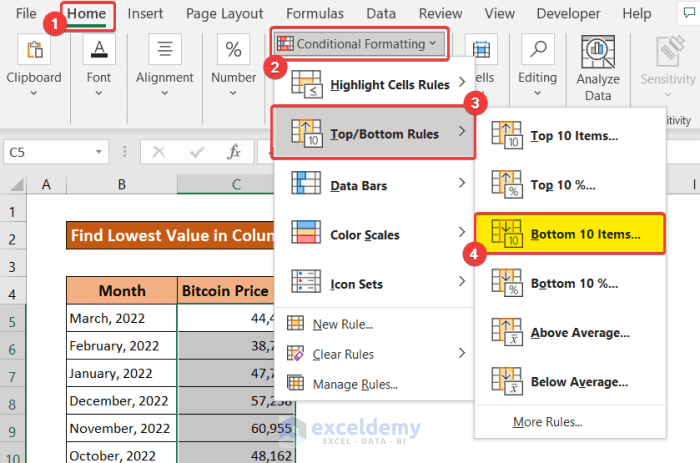
- Select the column you want to format.

- In the Home tab, under the Styles group, select Conditional Formatting.
- Select Top/Bottom Rules, and then select Bottom 10 Items.
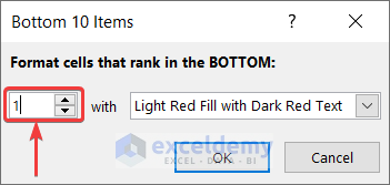
- In the Bottom 10 Items box that pops up, select or write the value 1.
- Click on OK.
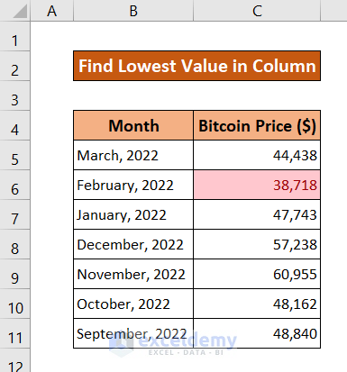
- Excel will highlight the lowest value.
Method 6 – Lookup the Lowest Value in an Excel Column
Let’s show during which month Bitcoin had the lowest price.
Steps:
- Find a minimum value using one of the first three methods and put it cell F5.
- Select the result cell F6.
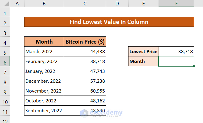
- Use in the following formula.
=INDEX(B5:B11,MATCH(MIN(C5:C11),C5:C11,0))- Press Enter.
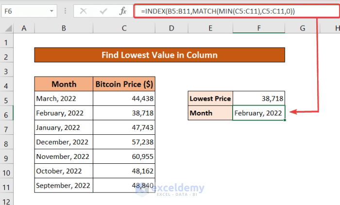
Breakdown of the formula:
- MIN(C5:C11) finds the lowest value from the range C5 to C11, in this case, it is 38,718.
- MATCH(MIN(C5:C11), C5:C11,0) finds the row number where 38,718 is located from C5 to C11, which is 2.
- INDEX(B5:B11, MATCH(MIN(C5:C11), C5:C11,0)) will show the value of the 2nd cell from range B5:B11, February 2022.
Download the Practice Workbook
Related Articles
- How to Find Last Row with a Specific Value in Excel
- How to Find Last Non Blank Cell in Row in Excel
- How to Find Last Cell with Value in Column in Excel
- Excel Find Last Column With Data
- How to Use Excel Formula to Find Last Row Number with Data
- How to Find Last Cell with Value in a Row in Excel
<< Go Back to Find Value in Range | Excel Range | Learn Excel
Get FREE Advanced Excel Exercises with Solutions!

