Method 1 – Applying a Combined Formula
Steps
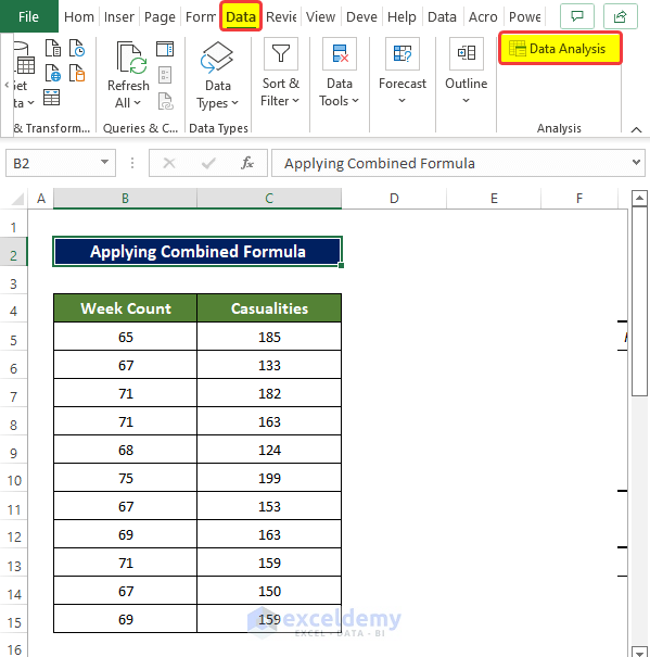
- Go to Data and select Data analysis.
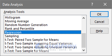
- Select the option Regression.
- Click OK.
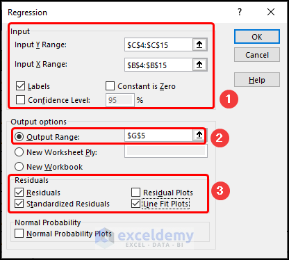
- In the Input Y Range box, select the range of cells C4:C15.
- In the Input X Range box, select the range of cells B4:B15.
- Check the Labels box.
- In the Output options group, select the Output Range and put cell G5 in the range box.
- Check the Residuals, Standardize Residuals, and Line Fit Plots boxes.
- Click OK.
- The Regression Analysis results are now presented in the Excel sheet starting from the G5 cells.
We will need the Squared Sum value of the residuals and will use that value to calculate the Standard Deviation of the residuals.
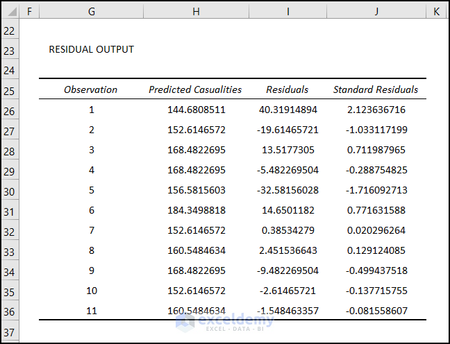
- Select the cell K26 and enter the following formula:
=I26^2This will calculate the square of the residual at cell K26.
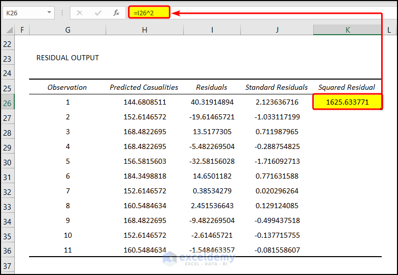
- Drag the Fill Handle to cell K36.
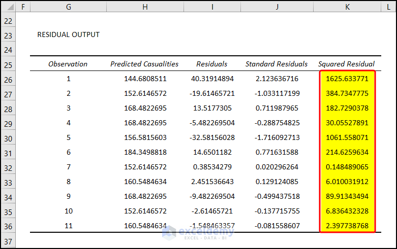
- Select the cell K37 and enter the following formula:
=SUM(K26:K36)- This will calculate the Sum of the Squared Residuals (SSE).
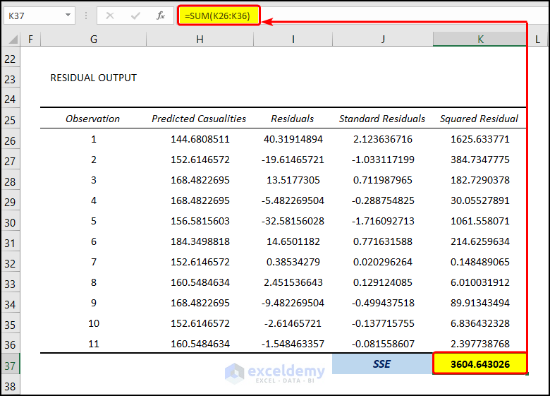
- To calculate the Standard Deviation(S), select the cell K38 and enter the following formula:
=2*SQRT(K37/(H10-2))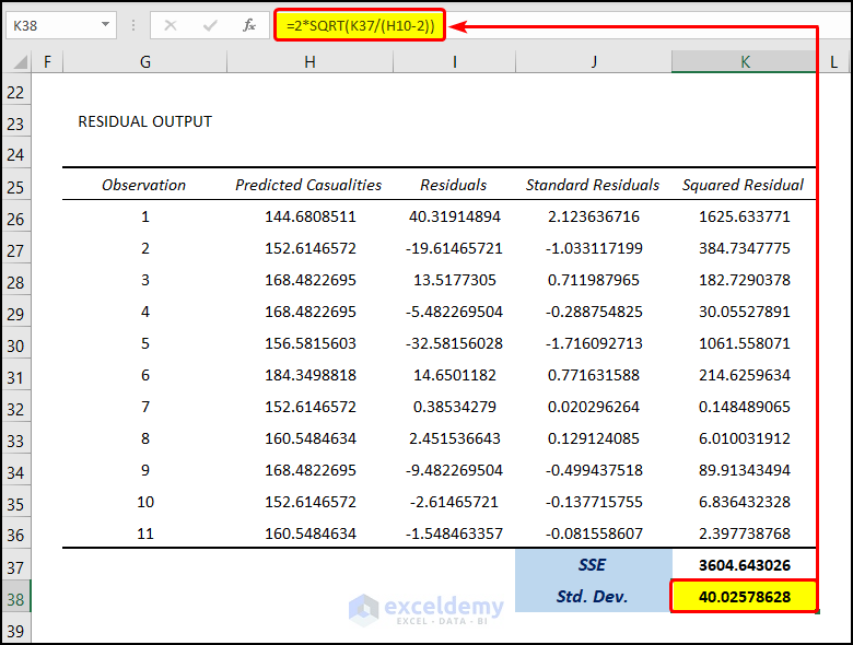
- This value is the value of the Standard Deviation of the residuals of the given dataset.
- Select the cell L26 and enter the following formula:
=IF(ABS(I26)>$K$38,"Outlier","Not Outlier")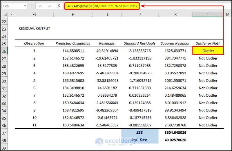
- This formula will check whether the absolute value of the residuals is greater than the Sum of the Squared Residuals(SSE) calculated in the earlier step. If the residual is greater than the SSE value, the cell will show “Outlier”. Otherwise, it will show “Not Outlier”.
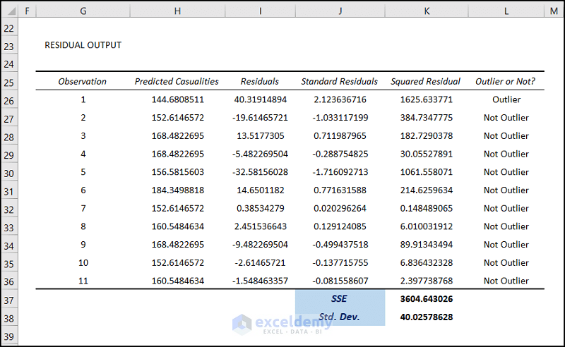
- Drag the Fill Handle to the cell L36.
- The first value of the range of cell L26:L36 is showing Outlier. The rest of them are Not Outliers.
- Select the cell D5 and enter the following formula:
=C5+$K$38 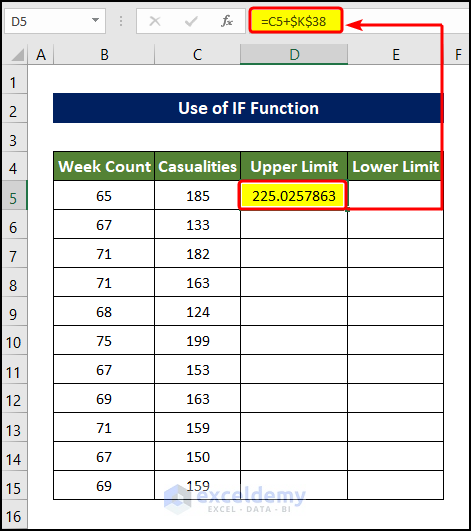
- Drag the Fill Handle to cell D15, which will fill the range of cell D5:D15 with the upper limit of the casualties Outlier value. Any value above the values will be considered an Outlier.
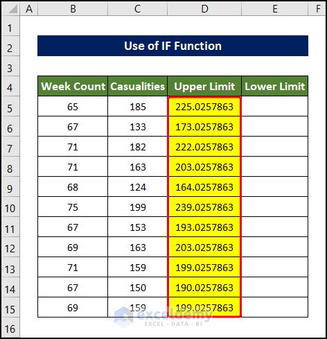
- Select cell E5 and enter the following formula:
=C5-$K$38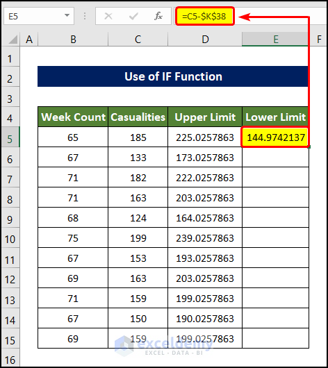
- Drag the Fill Handle to cell E5. This will fill the range of cell E5:E15 with the lower limit of the Outlier value of Casualties.
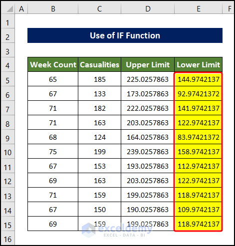
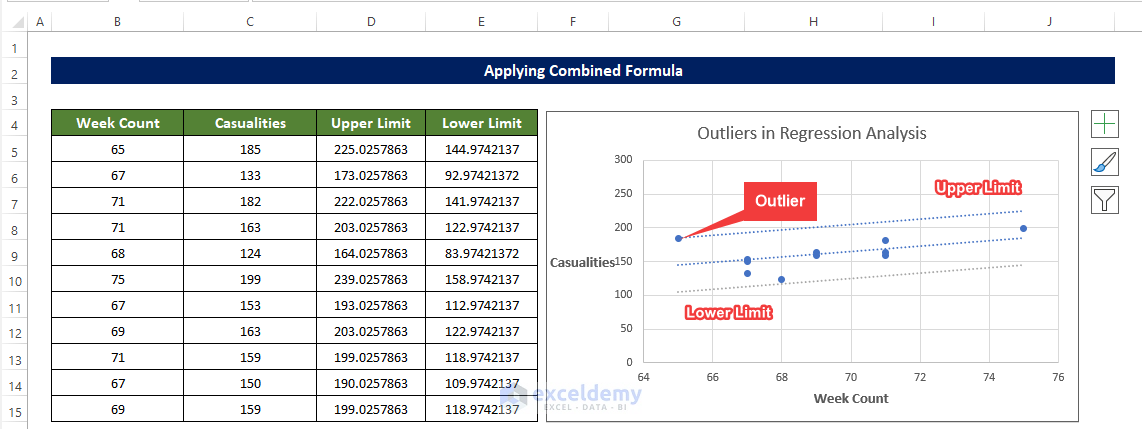
- We created the graph with the values we obtained so far, which constitutes the lower and the upper limit of the Outlier values.
Read More: How to Calculate Outliers in Excel
Method 2 – Applying the Inter-Quartile Range
Steps
- Select the cell F5 and enter the following formula:
=QUARTILE.EXC(C5:C11,1)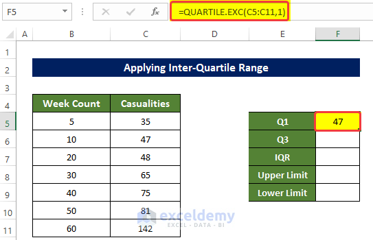
- Select the cell F5 and enter the following formula:
=QUARTILE.EXC(C5:C11,3)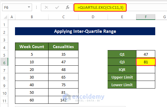
- Select the cell F7 and enter the following formula:
=F6-F5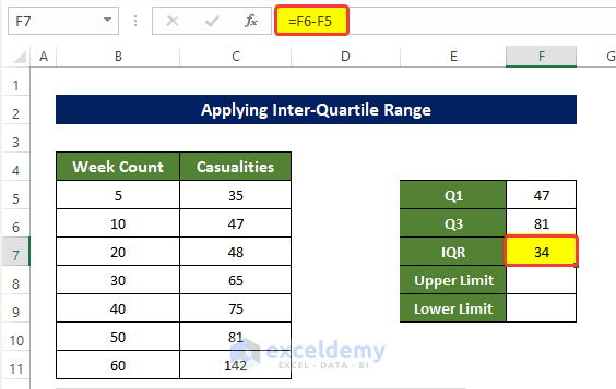
- Select the cell F8 and enter the following formula:
=F6+1.5*F7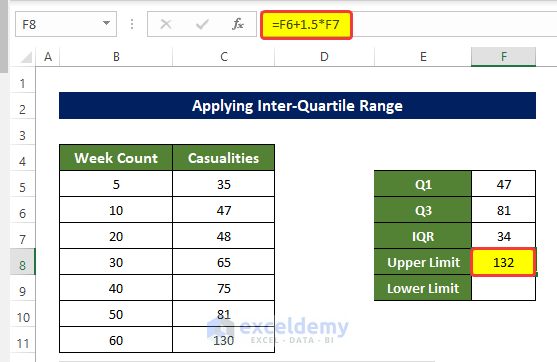
- Select the cell F9 and enter the following formula:
=F5-(F7*1.5)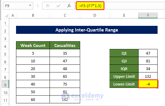
- Select the cell D5 and enter the following formula:
=IF(C5<G9,"Outlier","Not Outlier")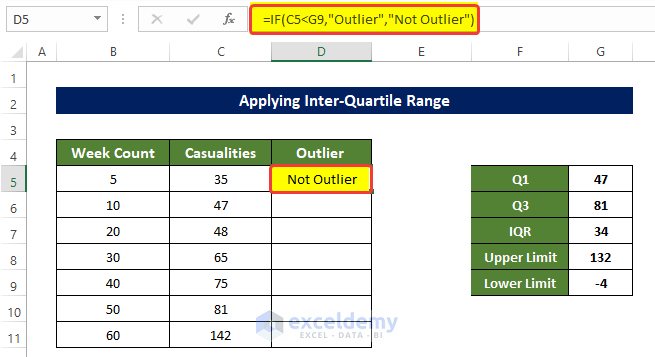
- Drag the Fill Handle to cell D11.
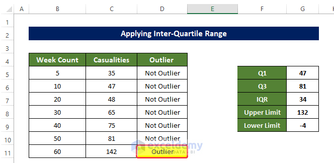
- This will fill the range of cell D5:D11 with text indicating whether the value is an Outlier.
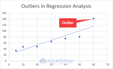
- We created a scatter plot of the graph.
Read More: How to Show Outliers in Excel Graph
Method 3 – Using Charts to Find Outliers
Steps
- Go to the Insert tab and click on Scatter in the Charts group.
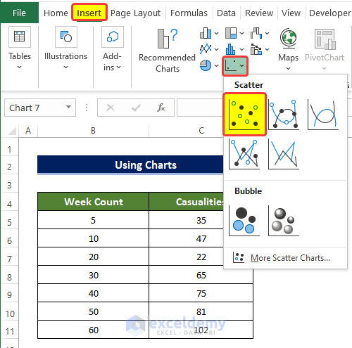
- Right-click on the chart and click on Select Data.
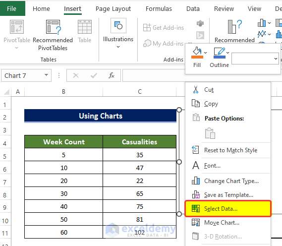
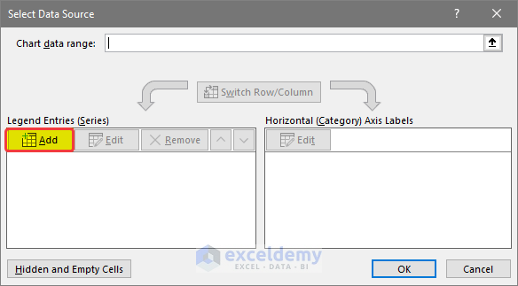
- You will get a new dialog box named Select Data Source.
- Click on the Add button.
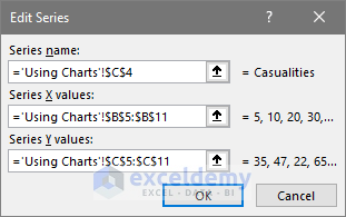
- In the Edit Series dialog box, click on the Series X values range box and select the range of cells B5:B11.
- Click on the Series Y value range box and select the range of cells C5:C11.
- Click OK.
- The chart in the worksheet now has the data plotted.
- Click on the plus icon on the right side of the chart.
- Choose and tick the Trendline box.

- Double-click on the Trendline to select it and then right-click on it.
- Click on Format Trendline.
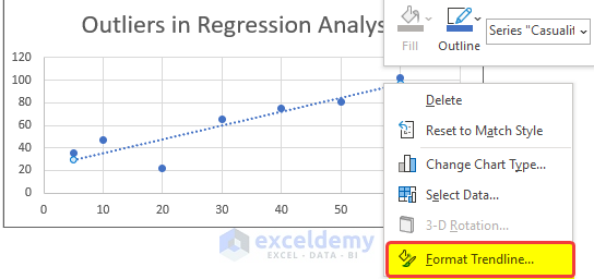
- Tick the Display Equation on chart and the Display R Squared value boxes.
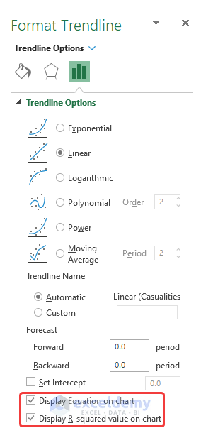
- The equation and the r-squared value of the equations are now presented in the chart.
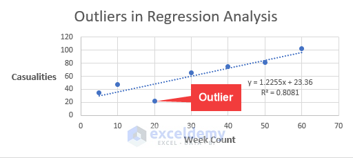
- From the chart, it is quite evident the third value in the database is the Outlier, as it is quite away from the Trendline.
Note
This method only works when the dataset is small, where you can scan the value and the chart quickly. In a large dataset, you should opt for other methods.
Read More: How to Find Outliers with Standard Deviation in Excel
Download the Practice Workbook
Related Articles
<< Go Back to Outliers in Excel | Excel for Statistics | Learn Excel
Get FREE Advanced Excel Exercises with Solutions!


This is very hard to follow for setting up with your own dataset. The column values are not consistent, so it is hard to know what you should be applying across different columns. The standard deviation calculation references G10 – but there is nowhere where G10 is referenced! The formula is also not the standard deviation formula I am familiar with, which has N on the bottom. Doing the maths to work out what G10 is – it is 9 – but there is NO VALUE 9 anywhere above – so it is very confusing. I’ve tried a number of different ways to work this out, and every time, either all my points are outliers or all are not. The graph it is very easy to see that there are outliers – but this regression method is very complicated to follow!
Hello KAREN W,
First of all, we would like to apologize for the trouble. As you pointed out, there were in fact some issues with the cell referencing in the Regression mathod, luckily they have been updated.
The Exceldemy team is grateful to you for sharing your thoughts and feedback. Hopefully, now you can obtain the desired result.