How to Find Repeated Cells in Excel: 4 Easy Methods

Method 1 – Applying Excel Conditional Formatting to Find Repeated Cells

Steps:

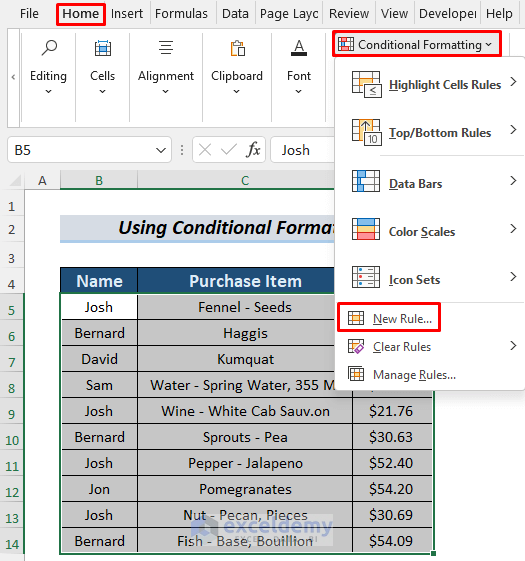
• Select the range B5:D14 and go to Home >> Conditional Formatting >> New Rule.

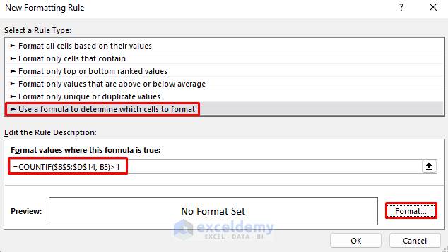
• The New Formatting Rule window will show up. Sselect ‘Use a formula to determine which cells to format’.
• Type the following formula in the ‘Format values where this formula is true’ section.

• Click Format.

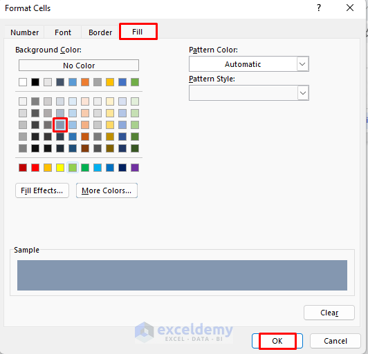
• The Format Cells window will show up. Select Fill and choose a color.
• Click OK.

• The New Formatting Rule window will appear again. Just click OK.

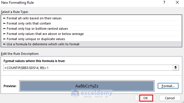
You will see all the repeated cells are filled with the selected color.

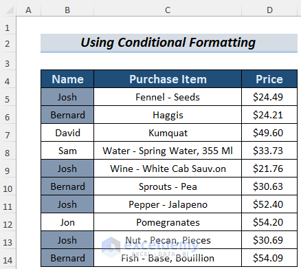
Find repeated cells in Excel using the Conditional Formatting application.

Method 2 – Using IF and COUNTIF Functions to Find Repeated Cells.

Steps:

• Make a new column to identify whether a repeat occurs, and type the following formula in cell E5.

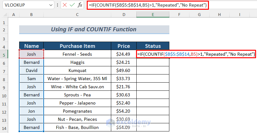
The formula here returns Repeated if the name in B5 is found more than once in the B5:B14 range and No Repeat if the name is found only once. The COUNTIF function counts the number of times these names appear in the range and the IF function tests whether that number is greater than 1. If the logical_test of the IF function is TRUE, then it will return Repeated, otherwise it will return No Repeat.

• Press the ENTER button and you will see if the name in B5 occurs more than once or not.

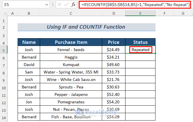
• Use the Fill Handle to AutoFill the lower cells.

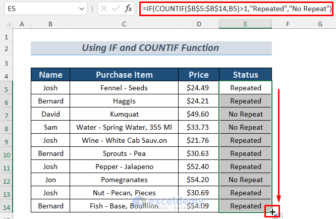
You will be able to find the repeated cells by using IF and COUNTIF functions.

Method 3 – Implementing Excel TEXTJOIN Function for Repeated Cells of Rows

Steps:

• Make a column to store the data of the cells in a row as a complete package and type the following formula in E5, press ENTER and drag the Fill icon downwards to AutoFill the lower cells.

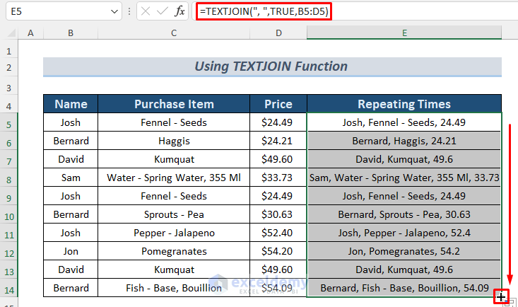
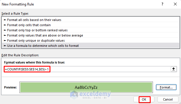
• Select the range B5:E14, open the New Formatting Rule window as we did in Method 1, and type the following formula in the ‘Format values where this formula is true’ section. Select a Format Cell color of your choice.

• Click OK.

The repeated rows will be highlighted after the execution of this command.

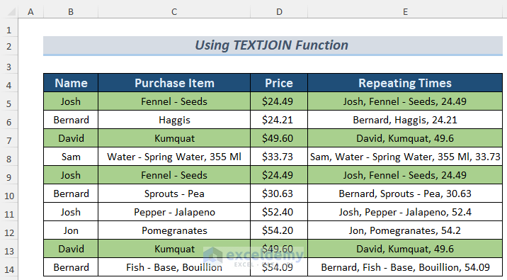
Thus you can find repeated cells by using the TEXTJOIN function.

Method 4 – Finding Repeated Cells Without Formulas

Steps:

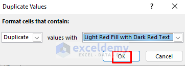
• Select the range B5:B14 and then go to Home >> Conditional Formatting >> Highlight Cell Rules >> Duplicate Values.

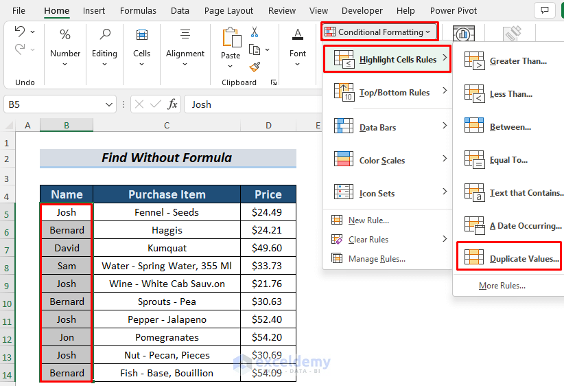
• A dialog box will appear. Click OK.

• You will see that this operation highlights the repeated cells in the range B5:B14.

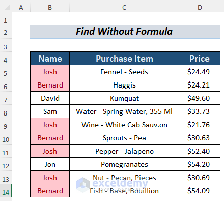
You can find repeated cells in Excel without using any formula.

Download Practice Workbook

Related Articles

• How to Compare Two Excel Sheets for Duplicates
• How to Find Matching Values in Two Worksheets in Excel
• How to Find Duplicates in Excel and Copy to Another Sheet
• Excel VBA to Find Duplicate Values in Range
• How to Find Duplicates in a Column Using Excel VBA
• How to Use VBA Code to Find Duplicate Rows in Excel

<< Go Back to Duplicates in Excel | Learn Excel