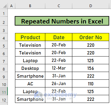
To demonstrate our methods, we’ll use the following dataset, which contains some Products and their Order no along with the Date. Some numbers are repeated. Let’s find them.
1. Using COUNTIF Function
Steps:
- In cell E5 enter the following formula:
=COUNTIF($D$5:$D$12,D5)>1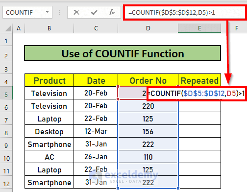
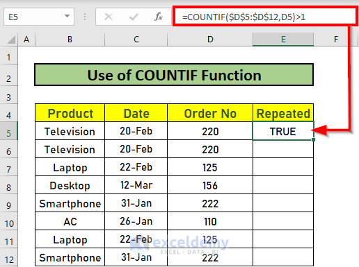
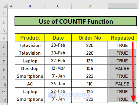
Our formula will find if the number in D5 is repeated in the range D5:D12. In case of repetition, Excel will return TRUE as output, else the output will be FALSE.
- Press ENTER to return the output.
- Use the Fill Handle to AutoFill down to cell D12.
Read More: How to Find Duplicate Rows in Excel
Method 2 – Using a Combination of IF and COUNTIF Functions
Steps:
- In cell E5 enter the following formula:
=IF(COUNTIF($D$5:$D$12,D5)>1,"Repeated","")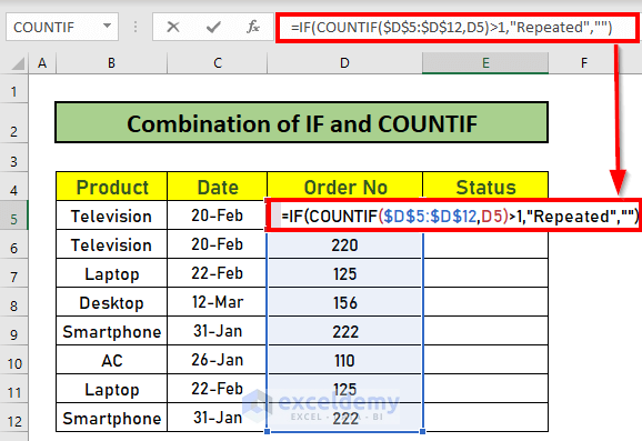
Formula Breakdown:
- COUNTIF($D$5:$D$12,D5)>1 → This is the logical test, which returns TRUE, since 220 is present more than once in D5:D12.
- =IF(COUNTIF($D$5:$D$12,D5)>1,”Repeated”,””) → If the test is TRUE, “Repeated” is returned, else a blank cell.
- Output: Repeated.
- Press ENTER.
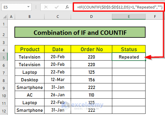
- Use Fill Handle to AutoFill down to D12.
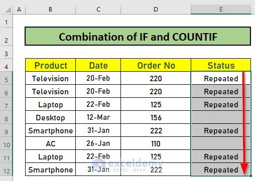
Read More: How to Find Repeated Cells in Excel
Method 3 – Find Repeated Numbers Without Mentioning the First Case
Steps:
- In E5 enter the following formula:
=IF(COUNTIF($D$5:$D5,D5)>1,"Duplicate","")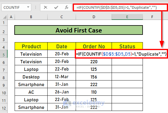
This formula will determine whether the number in D5 is repeated or not in D5:D12. Since this is the first case of 220, Excel will ignore it and the output will be blank.
- Press ENTER to return the output.
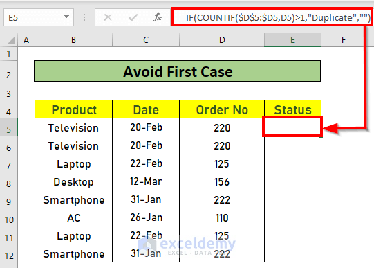
- Use the Fill Handle to AutoFill down to D12.
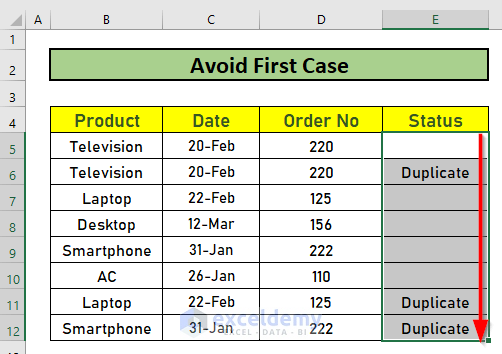
Notice that Excel returns “Duplicate” in E6. That’s because this is the second case. As mentioned earlier, for the first case, Excel will return a blank.
Read More: How to Filter Duplicates in Excel
Method 4 – Using Conditional Formatting
Steps:
- Select cells D5:D12.
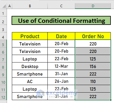
- Go to the Home tab.
- Select Conditional Formatting.
- Select Highlight Cell Rules.
- Select Duplicate Values.
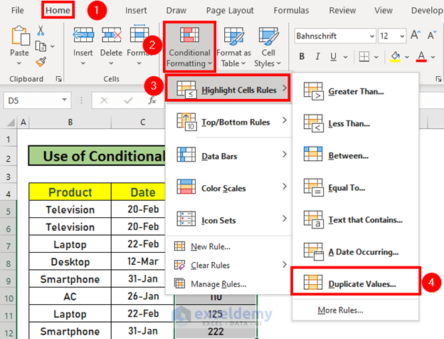
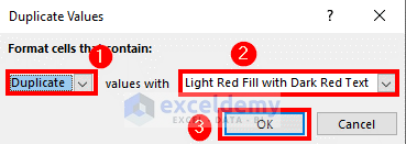
A Duplicate Values box will appear.
- Set Duplicate values to be formatted with Light Red Fill with Dark Red Text.
- Press OK.
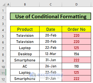
Excel will format the cells accordingly.
Read More: How to Compare Rows for Duplicates in Excel
Method 5. Using a Pivot Table
Steps:
- Select the entire dataset.
- Go to the Insert tab.
- Select PivotTable.
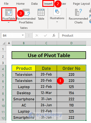
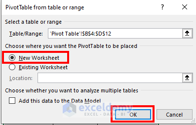
A box will pop up.
- Select New Worksheet to create a pivot table in a new worksheet.
- Press OK.
Excel will create a pivot table.

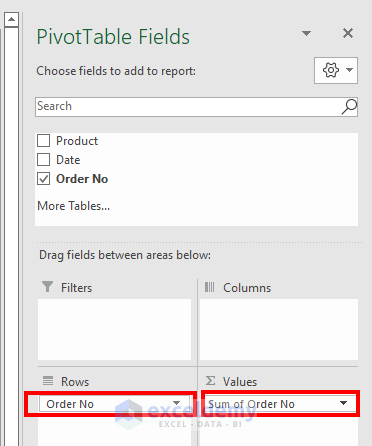
- Drag Order No to Rows and Values.
Excel will by default place Sum of Order No in the Values field, which we will modify below.
- Select the drop-down (see image below).
- Select Value Field Settings.
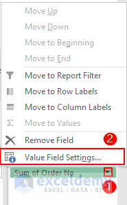
The Value Field Settings box will pop up.
- Select Count.
- Press OK.
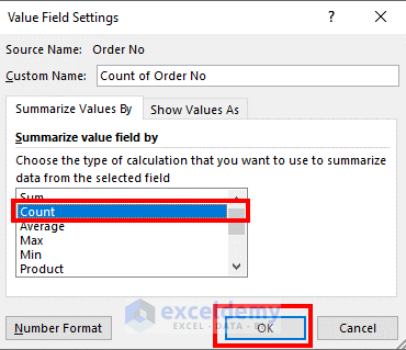
Excel will count the Order Numbers.
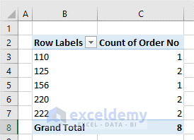
The returned result: 125, 220, and 222 are repeated numbers.
Read More: Excel Find Duplicate Rows Based on Multiple Columns
Things to Remember
- Use absolute reference to lock a cell.
- If you have earlier versions of Excel, you may need to press CTRL+SHIFT+ENTER for array formulas.
Download Practice Workbook
Related Articles
- How to Compare Two Excel Sheets for Duplicates
- How to Find Matching Values in Two Worksheets in Excel
- How to Find Duplicates in Excel and Copy to Another Sheet
- Excel VBA to Find Duplicate Values in Range
- How to Find Duplicates in a Column Using Excel VBA
- How to Use VBA Code to Find Duplicate Rows in Excel
<< Go Back to Find Duplicates in Excel | Learn Excel
Get FREE Advanced Excel Exercises with Solutions!

