Microsoft Excel computes costs associated with our mortgages, such as interest and monthly payments, which is one of its powerful features. If you are a little familiar with Excel functions, building a fixed rate mortgage calculator in Excel is simple. In this article, we will learn 5 easy steps to create a fixed rate mortgage calculator in Excel.
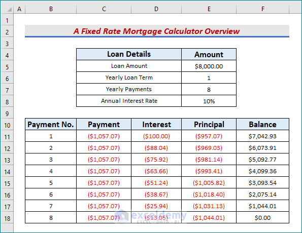
Before diving into the methods in the next section, let’s take a look at the screenshot that represents the overview of a fixed-rate mortgage calculator in Excel.
Introduction to Fixed Rate Mortgage
A house loan with a fixed interest rate for the duration of the loan is referred to as a Fixed Rate Mortgage. The Fixed Rate indicates that the interest rate on the mortgage remains the same throughout. For customers who want to know how much they will pay each month, Fixed Rate Mortgages are attractive options. Some key points:
- The majority of fixed-rate loans amortize over time.
- Once fixed, changes in the market don’t affect the interest rate.
- Alternatively, mortgages with adjustable rates fluctuate in interest during the term of the loan.
How to Create Fixed Rate Mortgage Calculator in Excel (With Easy Steps)
Excel does not come with a built-in mortgage calculator. In order to build a mortgage calculator and compute the amortization loan table, we will use the PMT, IPMT, and PPMT functions in our spreadsheet. Moreover, we will utilize the Additional formula for calculation. A loan that is repaid in installments over the course of the loan’s term is simply referred to as an amortizing loan. So, without any further delay, let’s get straight to the steps.
Step 1: Introduce Dataset with Proper Parameters
The first step aims to create a dataset with correct information. Add the following headers in the below-mentioned columns.
- Initially, introduce the header Loan Details and sub-headers Loan Amount, Yearly Loan Term, Yearly Payments, and Annual Interest Rate in column C.
- Further, populate them with correct values.

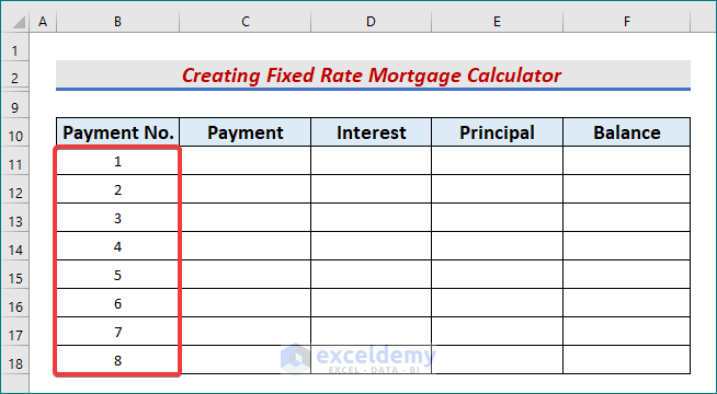
- Similarly, add the headers Payment No, Payment, Interest, Principal, Balance in B10, C10, D10, E10, and F10 respectively.
- Afterward, put a series of numbers up to B18 under Payment No.
Read More: Early Mortgage Payoff Calculator in Excel
Step 2: Utilize PMT Function to Calculate Total Payments
The objective of the second step is to utilize the PMT function to find the payments for each period. The PMT function uses a constant interest rate to determine how much a loan will cost. Follow the below instructions to understand better.
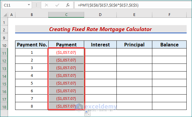
- Firstly, in cell C11, type the following formula:
=PMT($E$8/$E$7,$E$6*$E$7,$E$5)- Remember to use absolute cell references for these steps.
- Later, press the Enter or Tab keys to get the output.
- The formula’s output will be red, formatted as Currency, and rounded to two decimal places. When the result is automatically surrounded in parenthesis, it indicates that the loan amount is negative because the loan payment will be subtracted from the bank account.
- Put a minus (–) sign before the PMT function if you wish to see the positive loan amount.

- Meanwhile, use the AutoFill tool to drag the formula cell down.
- Thus, we obtain the fixed payments over the 8 periods.
Step 3: Apply IPMT Function to Determine Interests
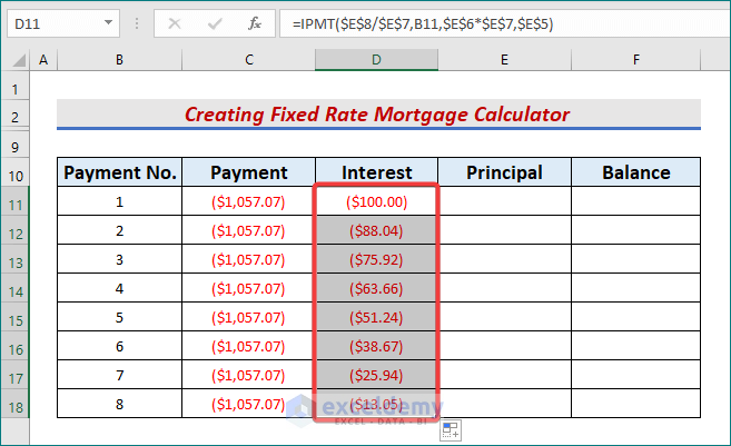
In the third step, we will thoroughly implement the IPMT function to calculate the interests over the 8 periods. Based on periodic, constant payments and a constant interest rate, the IPMT function returns the interest payment for a specified term for an investment. Let’s learn more about the following procedures.
- To begin with, write the formula in D11,
=IPMT($E$8/$E$7,B11,$E$6*$E$7,$E$5)- Here, C8 is the annual Interest rate, and 8 is the period for which we wish to calculate the interest payment. E7 is the total number of payments during the whole period and E5 is the present value of the loan.
- Pressing Enter will return the output.
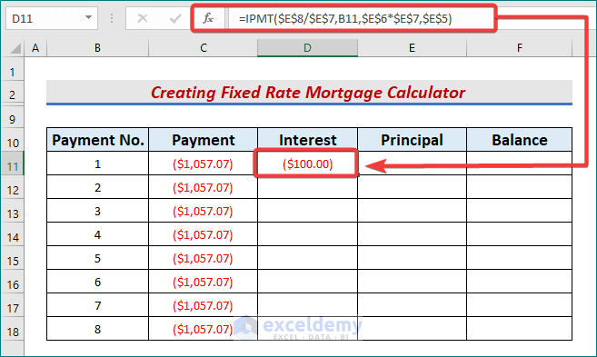
- Again, use the AutoFill icon to fill the rest of the column.
Read More: Mortgage Calculator with Extra Payments and Lump Sum in Excel
Step 4: Use PPMT Function to Count Principal
In our fourth step, we will calculate the principles using the PPMT function. For a given period, the PPMT function returns the principal payments. To demonstrate, follow the below instructions.
- Type the PPMT formula in cell E11,
=PPMT($E$8/$E$7,B11,$E$6*$E$7,$E$5)- $E$8/$E$7; declares rate/nper as an annual capital payment is calculated. It can also be a weekly (rate/52), or monthly (rate/12) payment.
- Next, press Enter or Tab.
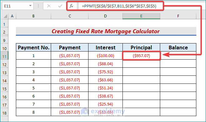
- After that, drag the formula cell down using the AutoFill tool.

Read More: Biweekly Mortgage Calculator with Extra Payments in Excel
Step 5: Insert Excel Formulas to Find Remaining Balance
In our last step, we will use 2 formulas to find the remaining balance after each period. Learn more about the formulas in the steps below.
- Firstly, in cell F11, type:
=E5+E11- This adds the Loan Amount with the first obtained Principal number.
- Now, press Enter to get the balance after the first payment.
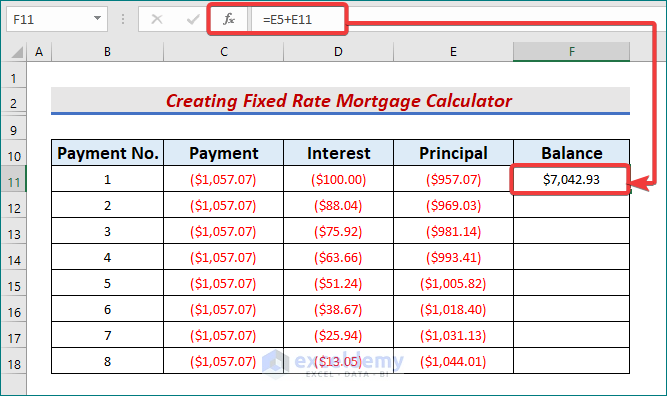
- Secondly, in F12:
=F11+E12- This adds up to the first balance and the second principal payment.
- Press Enter.
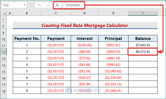
- Lastly, use the AutoFill tool until the balance becomes 0.
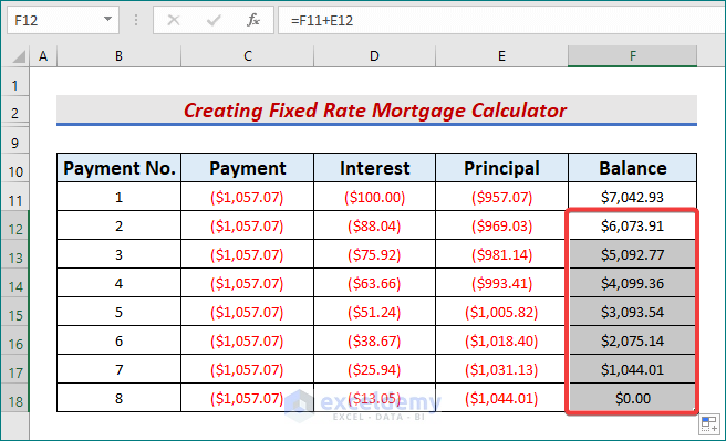
- Thus, we obtain our desired mortgage calculator for a fixed rate loan.
Read More: How to Create Offset Mortgage Calculator in Excel
Download Practice Workbook
Download this workbook and practice while going through the article.
Conclusion
In conclusion, we have discussed some easy steps to create a fixed-rate mortgage calculator in Excel. Please, leave any further queries or recommendations in the comment box below.
Related Articles
- Mortgage Repayment Calculator with Offset Account and Extra Payments in Excel
- How to Make Chattel Mortgage Calculator in Excel
- How to Create Reverse Mortgage Calculator in Excel
- Calculator for Effective Interest Method of Amortization
- Creation of a Mortgage Calculator with Taxes and Insurance in Excel
- Interest Only Mortgage Calculator with Excel Formula
<< Go Back to Mortgage Calculator | Finance Template | Excel Templates
Get FREE Advanced Excel Exercises with Solutions!

