How to Use a Formula to Find Bold Text in Excel (4 Methods)

Dataset Overview

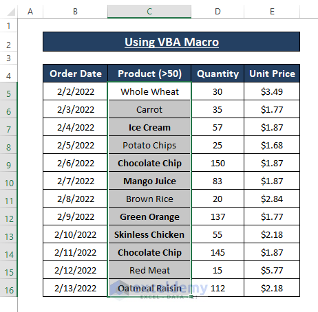
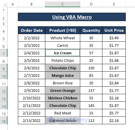
We’ll use a dataset that holds products sold on certain days. The products that have sold a Quantity of more than 50 (>50) are in bold. We have to find the bolden product names.

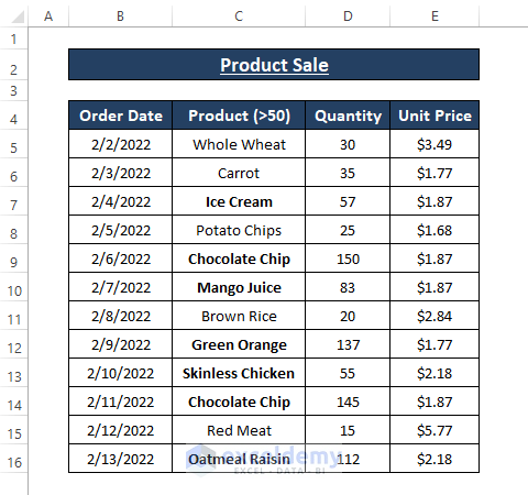
Method 1 – Using the Find Feature to Find Bold Text in Excel

Select the Range
- Choose the entire range (rows or columns) where you want to find bold text.
- Go to the Home tab and click on Find & Select (from the Editing section), then select Find.

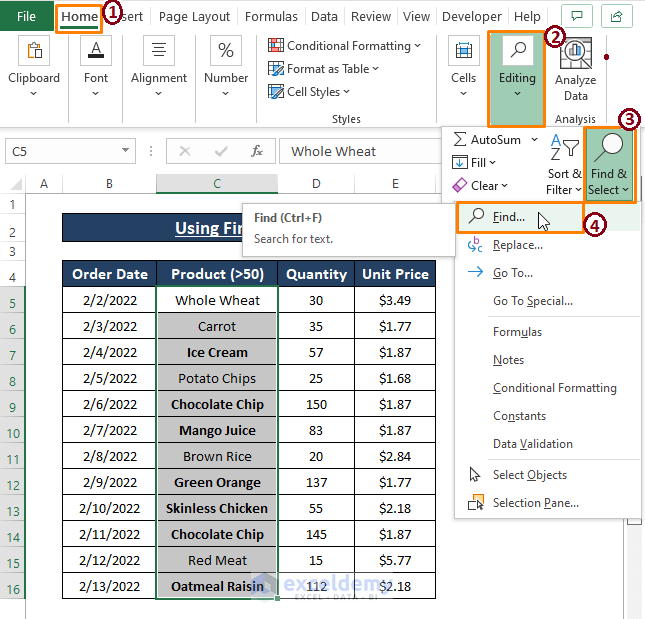
Find and Replace Dialog Box
- The Find and Replace dialog box appears.
- Keep other options as they are.
- Click on Format.

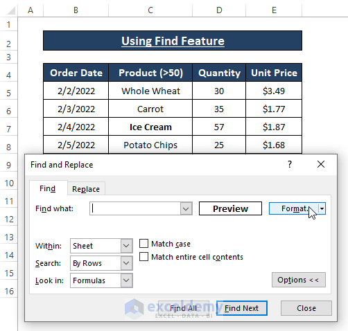
Find Format Dialog Box
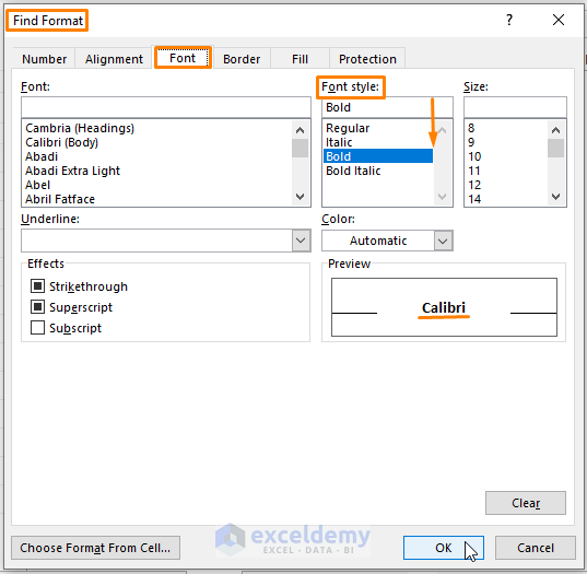
- In the Find Format dialog box:
  - Select the Font section.
  - Go to the Font Style group.
  - Choose Bold and click OK.

Find All Bold Text
- Click OK in the Find and Replace dialog box.
- All the bold texts within the selection will be listed under the dialog box.

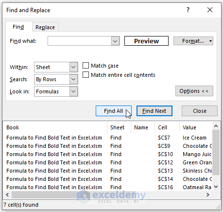
Select All Bold Text
- Press CTRL+A to select all the bold texts.
- Excel will highlight all the bold texts within your selection.

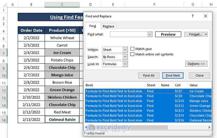
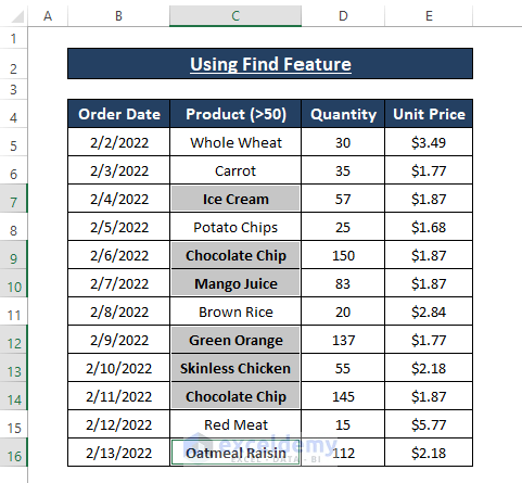
Read More: How to Find Text in Cell in Excel

Method 2 – Using the GET.CELL Formula to Find Bold Text

GET.CELL is a macro function that returns TRUE or FALSE depending on the types of cell information. The syntax of the GET.CELL is

GET.CELL(type_num, reference)

In the syntax,

type_num; is a number that indicates what type of cell info you consider finding. For this case type_num 20 refers to the first or all the characters of an entry in Bold font.

reference; cell reference.

Follow these steps to execute this method:

Define a Name
- Highlight the entire column containing the data.
- Go to the Formulas tab and select Define Name (from the Defined Names section).

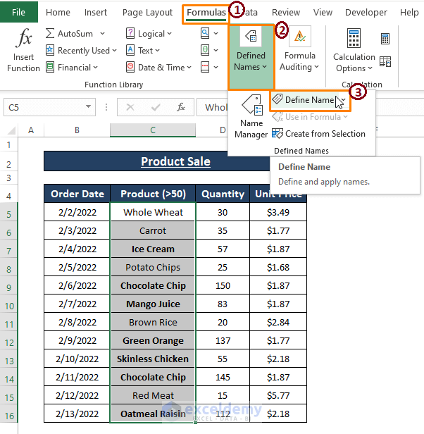
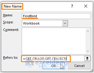
- In the New Name dialog box:
  - Assign a name (e.g., FindBold) to the range (Product column).
  - Set the following formula in the Refer to field:

=GET.CELL(20,GET.CELL!$C5)

Here, 20 represents the type_num for bold font or characters, and GET.CELL!$C5 is the reference.

Apply the Formula
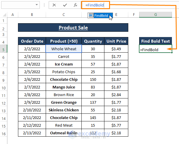
- Enter =FindBold in any blank cell (e.g., G5).
- Double-click on the defined name that appears under the formula bar.

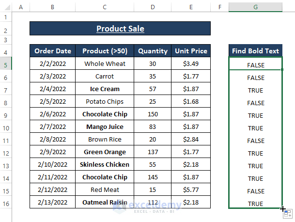
- Press ENTER and drag the Fill Handle to apply the formula to other cells.
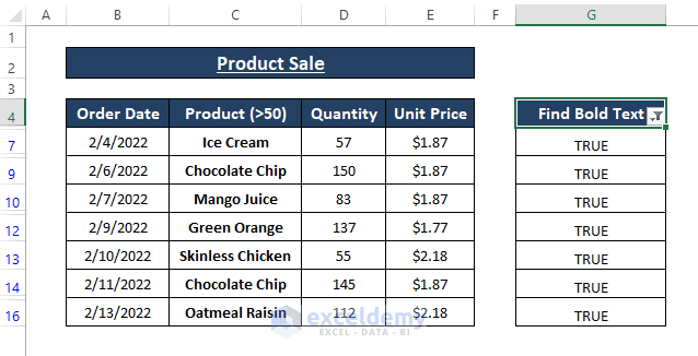
- Excel will display TRUE for bold entries and FALSE for non-bold entries.

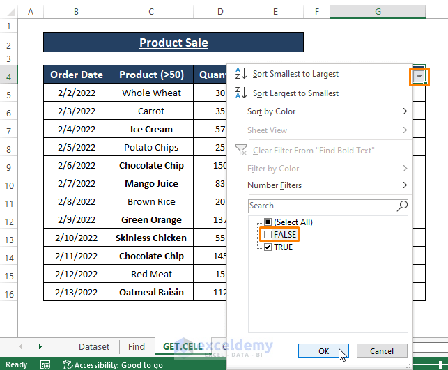
Filter Bold Entries
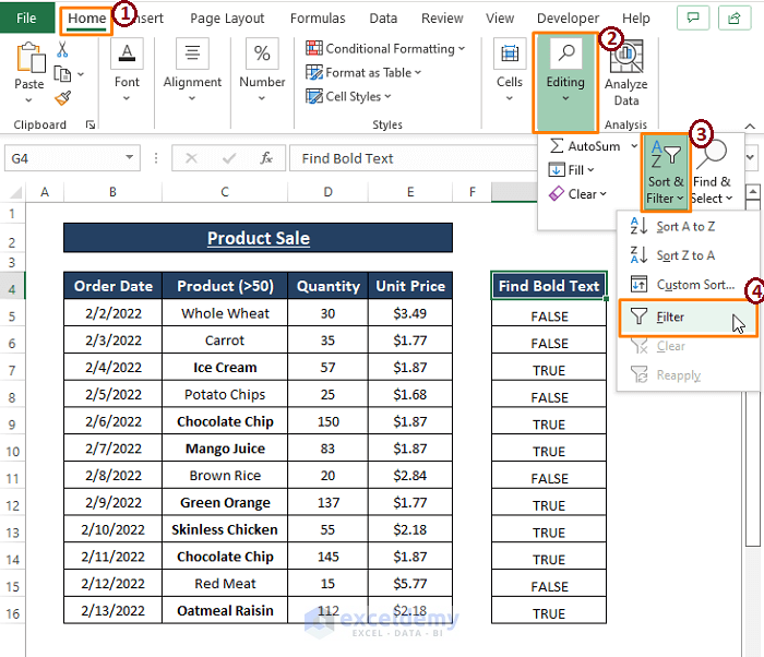
- Place the cursor on the header (Find Bold Text).
- Go to the Home tab, select Sort & Filter (from the Editing section), and click on Filter.

- Deselect FALSE in the Filter options and click OK.

- This will display all the bold entries and hide non-bold ones.

Read More: How to Get Excel Sheet Name

Method 3 – Using VBA Custom Formula to Find Bold Text

Open the Visual Basic Editor
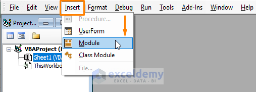
- Press ALT+F11 to open the Microsoft Visual Basic for Applications (VBA) window.
- In the window, select Insert from the toolbar and click on Module.

Create the Custom Function
- Paste the following macro into the module:

Function FindBold(wrkRng As Range)
If wrkRng.Font.Bold Then
FindBold = wrkRng.Value
Else
FindBold = ""
End If
End Function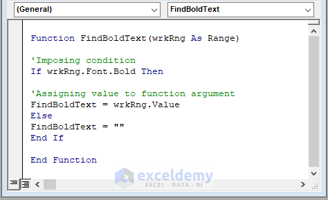

This custom function, named FindBoldText, takes a range as an argument. It checks if each cell’s font is bold and returns the cell value or an empty string accordingly.

Apply the Custom Formula
- Back in the worksheet, enter =FindBoldText in the formula bar.
- A custom formula with the same name as in the macro will appear. Double-click on it.

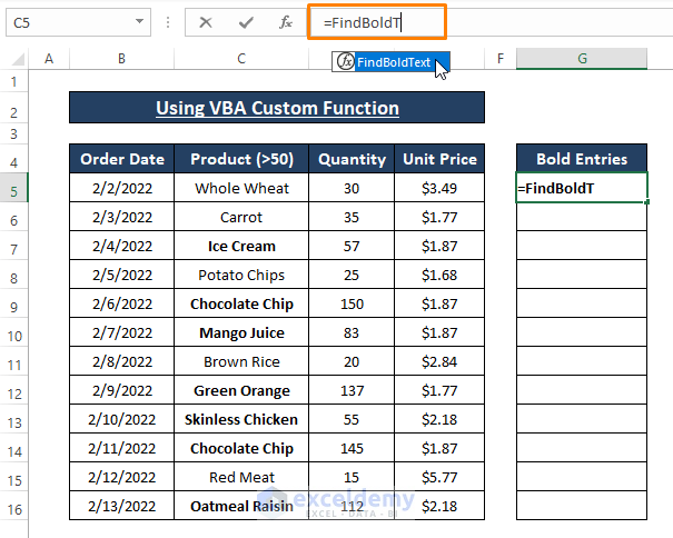
- Assign a cell as a reference and press ENTER.

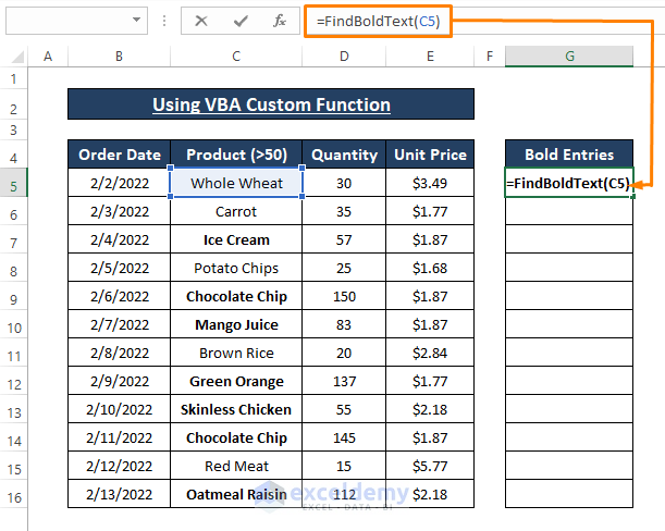
- Use the Fill Handle to apply the formula to other cells.

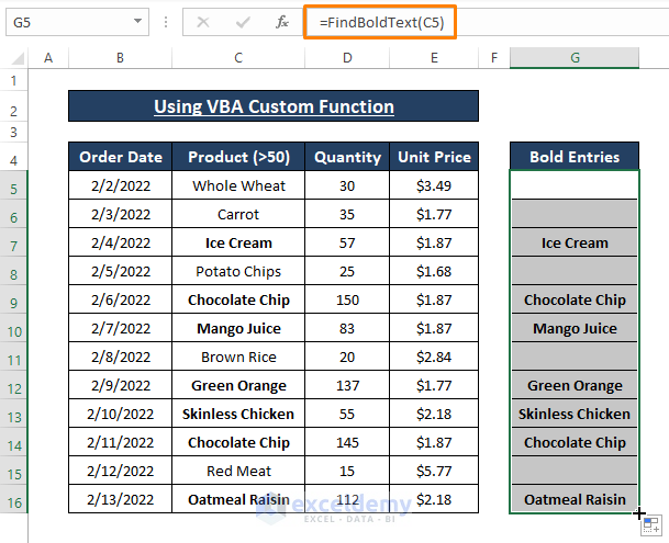
Filter Bold Entries
- Repeat Steps 5 and 6 from Method 2:
  - Apply a filter to the header (Find Bold Text).
  - Unselect Blanks from the filter options and click OK.

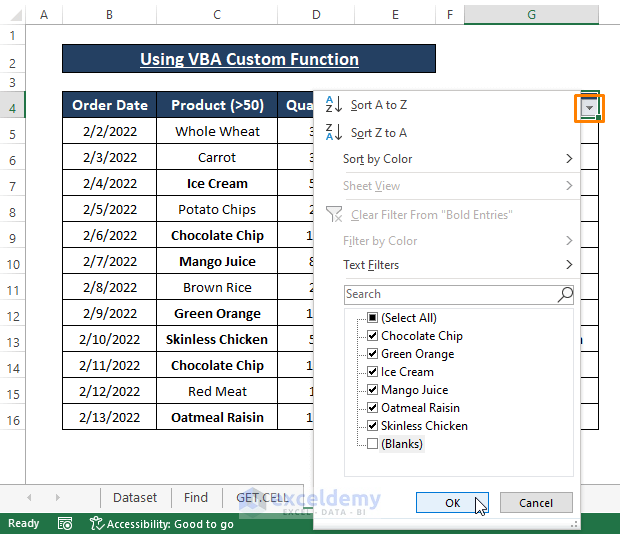
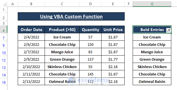
Excel will hide non-bold entries within the range, displaying only the bold ones.

Method 4 – Find Bold Text Using VBA Macro

Create a Simple Macro
- Select a range of cells.
- Press ALT+F11 to open the VBA window.
- Insert a module (similar to Step 1 in Method 3).

- Enter the following macro:

Sub FindBoldEntries()
Dim mrfRng As Range
Dim wrkRng As Range
Dim LRng As Range
On Error Resume Next
xTitleId = "Provide a Range"
Set wrkRng = Application.Selection
Set wrkRng = Application.InputBox("Range", xTitleId, wrkRng.Address, Type:=8)
For Each mrfRng In wrkRng
If mrfRng.Font.Bold Then
If LRng Is Nothing Then
Set LRng = mrfRng
Else
Set LRng = Union(LRng, mrfRng)
End If
End If
Next
If Not LRng Is Nothing Then
LRng.Select
End If
End Sub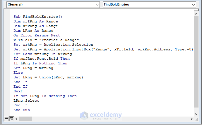

- This macro loops through the selected range, highlighting bold entries.

Run the Macro
- Press F5 to run the macro.
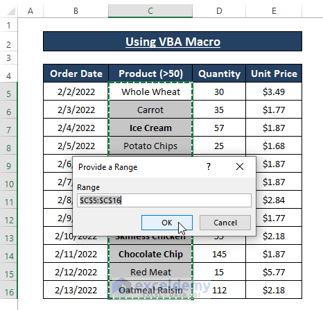
- Excel will automatically insert the selected range in the Provide a Range dialog box.
- Click OK.