[Solved] Vehicles Gas usage Summary

[Maps]

Good day.
I have a spreadsheet where I post gas issued to company vehicles.
The vehicles do not put in gas everyday. There are days when no gas is issued.
I have a sheet on spreadsheet which I call Sourcedata when I do the postings. I have created another sheet called Summary where I want to only show gas that has been issued.
How do I create a formula on the Summary sheet which will only show details of vehciles that were issued with Gas?
I have attached my spreadsheet.
I have mocked up the expected results on the summary sheet as attached.

 

[Lutfor Rahman Shimanto]

Good day.
I have a spreadsheet where I post gas issued to company vehicles.
The vehicles do not put in gas everyday. There are days when no gas is issued.
I have a sheet on spreadsheet which I call Sourcedata when I do the postings. I have created another sheet called Summary where I want to only show gas that has been issued.
How do I create a formula on the Summary sheet which will only show details of vehciles that were issued with Gas?
I have attached my spreadsheet.
I have mocked up the expected results on the summary sheet as attached.

Hello Maps

Thanks for reaching out and posting the exciting issue. Exploring the problem you mentioned, I understand you need help with an Excel formula to show details of vehicles that were issued with Gas. As you requested, I can assist you with a complex formula and implement that with the help of the SUM and VLOOKUP functions. To dynamically set the lookup range, you can improve the formula using the INDIRECT, IF and MAX functions.

The Formula Structure for All Cars:

=SUM(VLOOKUP(UNIQUE($A$12:INDEX($A:$A,MAX(IF($A$12:$A$28<>"",ROW($A$12:$A$28))))),SourceData!$A$12:$E$121, 4))

Exceptions for TATA NEW:

=SUM(VLOOKUP(UNIQUE(A12:A21),SourceData!A12:I121,8,FALSE))

I hope this will achieve your goal. I am also giving you the Workbook used to investigate your issue to help you understand better. Feel free to contact us again with any other inquiries or concerns.

Regards
Lutfor Rahman Shimanto

 

[Maps]

Hello Maps

Thanks for reaching out and posting the exciting issue. Exploring the problem you mentioned, I understand you need help with an Excel formula to show details of vehicles that were issued with Gas. As you requested, I can assist you with a complex formula and implement that with the help of the SUM and VLOOKUP functions. To dynamically set the lookup range, you can improve the formula using the INDIRECT, IF and MAX functions.

The Formula Structure for All Cars:



Exceptions for TATA NEW:



I hope this will achieve your goal. I am also giving you the Workbook used to investigate your issue to help you understand better. Feel free to contact us again with any other inquiries or concerns.

Regards
Lutfor Rahman Shimanto

Thanks Lutfor for your response.
However, what I am trying to do is to have the summary page pick the information from the sourcedata sheet where there are there gas issues and omit the the lines where there are no issues at all without changing the layout like I have done on the summary sheet.
The summary sheet is the expected result which I want a formula to pick from the sourcedata sheet.

 

[Lutfor Rahman Shimanto]

Thanks Lutfor for your response.
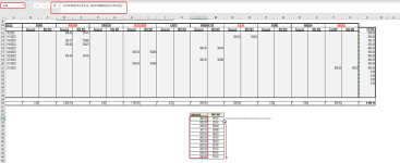
However, what I am trying to do is to have the summary page pick the information from the sourcedata sheet where there are there gas issues and omit the the lines where there are no issues at all without changing the layout like I have done on the summary sheet.
The summary sheet is the expected result which I want a formula to pick from the sourcedata sheet.

Dear Maps

Again, Thank you for reaching out and explaining the issue with clarity. You want to pick the information from the SourceData sheet where gas is issued and avoid the line with no gas issues. In the Summary sheet, you have written the expected result.

As requested, I have developed a formula using the SUMIFS function and tried only using the SourceData sheet to display the result. Here, the SUMIFS function will sum the values in the range SourceData!B12:B121 that correspond to the non-empty cells in SourceData!A12:A121.

=SUMIFS(SourceData!$D$22:$D$121,SourceData!$A$22:$A$121,"<>")

Likewise, I use the same formula for all car columns. I am attaching the solution workbook to help you understand better. Good luck.

Regards
Lutfor Rahman Shimanto

 

[Maps]

Good morning.
Thanks once again Lutfor for your response. I see you have given a formula that summarises the total gas issued per vehicle. I actual want the issues itemised on the summary page excluding cells where no gas has been issued in the sourcedata page.
1. The first issue being cell L17:M17 on the sourcedata. I need this to shown on cell L12:M12 of the summary sheet through a formula.
2. The first issue being cell D23:E23 on the sourcedata. I need this to shown on cell L13:M13 of the summary sheet through a formula.
etc.
The blank line to be embedded on the lines that have values.

 

[Lutfor Rahman Shimanto]

Good morning.
Thanks once again Lutfor for your response. I see you have given a formula that summarises the total gas issued per vehicle. I actual want the issues itemised on the summary page excluding cells where no gas has been issued in the sourcedata page.
1. The first issue being cell L17:M17 on the sourcedata. I need this to shown on cell L12:M12 of the summary sheet through a formula.
2. The first issue being cell D23:E23 on the sourcedata. I need this to shown on cell L13:M13 of the summary sheet through a formula.
etc.
The blank line to be embedded on the lines that have values.

Hello Maps

Thank you once again for explaining more about the problem. I still needed help understanding embedding new lines. Anyway, I understand the first issue in range L17:M17 of SourceData goes to L12:M12 in the Summary sheet using a formula. Likewise, the second issue in D23:E23 of SourceData goes to L13:M13 in the Summary sheet using a formula. This process repeats for other gas issues.

The requirement can be resolved by using two Helper columns. I apply the formula below on the Summary sheet in the X column, and it retrieves all non-empty cells for a row, and later I drag the fill handle icon to X122.

​

=FILTER(SourceData!B12:U12,SourceData!B12:U12<>"")

Calculation:

​

Next, I use the formula below in cell L34 (For Demonstration) to find only the numbers from the X column.

​

=FILTER(X12:X121, ISNUMBER(X12:X121))

After that, I utilize the VLOOKUP function in cell M34 and dragged the fill handle icon to M44 to get the Invoice no from the Y column.

​

=VLOOKUP(L34,$X$11:$Y$122,2,FALSE)

Result:

​

To help you better understand the situation, I'm also giving you the Workbook used to examine it. If you have any more queries or problems, do get in contact with us.

Regards
Lutfor Rahman Shimanto

 

[Maps]

Thanks once again Lutfor.
It seems what I was asking was a bit complicated and not quite possible. But thanks for trying so hard to help me.

 

[Lutfor Rahman Shimanto]

Thanks once again Lutfor.
It seems what I was asking was a bit complicated and not quite possible. But thanks for trying so hard to help me.

Dear Maps

You're most welcome! It was my pleasure to assist you. Sometimes, our challenges can be complex, and finding the perfect solution can be challenging. Indeed, the challenges can be made more accessible by utilizing Excel VBA.

Please don't hesitate to reach out again if you have further questions or need assistance. We are here to support you to the best of our abilities.

Regards
Lutfor Rahman Shimanto

 

[Maps]

Yes please.
Thank you once again Lutfor.