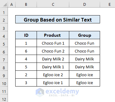
Method 1 – Row or Column-wise Grouping for Similar Items
Sometimes, we need to group similar items based on rows or columns. In this section, I’ll show you how to group similar items both row-wise and column-wise. Let’s assume we have a dataset containing information about people, including their addresses and purchased products. The columns in our dataset are as follows: Address, First Name, Last Name, and Product.
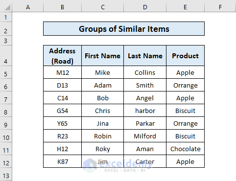
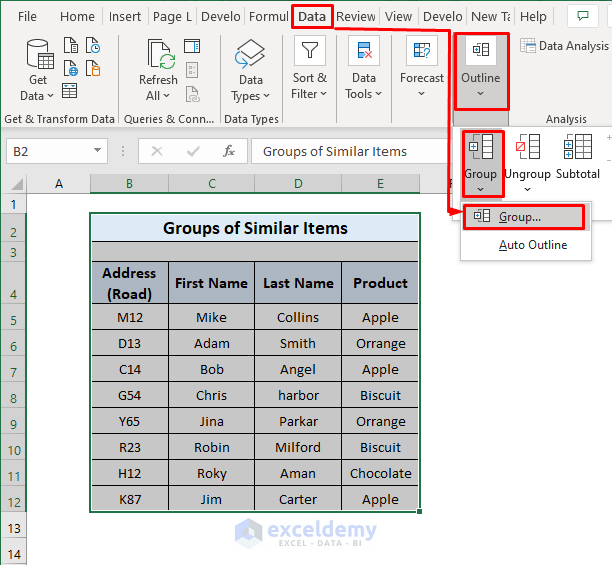
- Select the cells you want to group. These could be rows or columns containing related data.
- Go to the Data tab in Excel.
- Click the Group button.
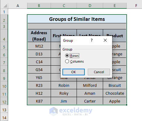
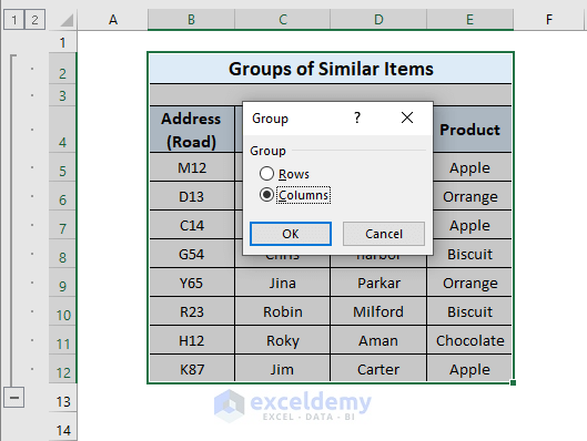
- Choose whether you want to group the rows or the columns.
- If you click on rows, your rows will be grouped together.
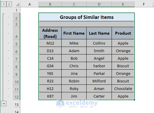
- Similarly, you can create a group based on columns.
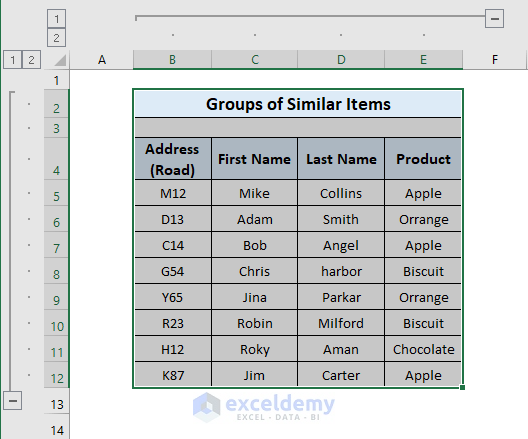
- Now you have grouped similar items. You can choose to either display or hide the group.
- Sometimes, you might need to hide certain data temporarily for further analysis. By grouping them, you can easily show or hide the relevant information.
Read More: How to Group Cells with Same Value in Excel
Method 2 – Grouping Cells with Same Items Using Excel’s Subtotal Feature
For the dataset from the previous method, let’s explore the application of the Subtotal feature. This method allows us to calculate the total count of similar items in Excel. Follow these steps:
- Choose the row or column that you want to categorize (e.g., the Product column).
- Go to the Sort & Filter section on the Home tab.
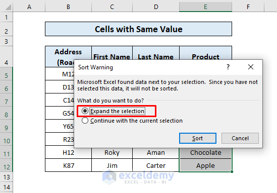
- Click Sort A to Z (or any other sorting option you prefer).
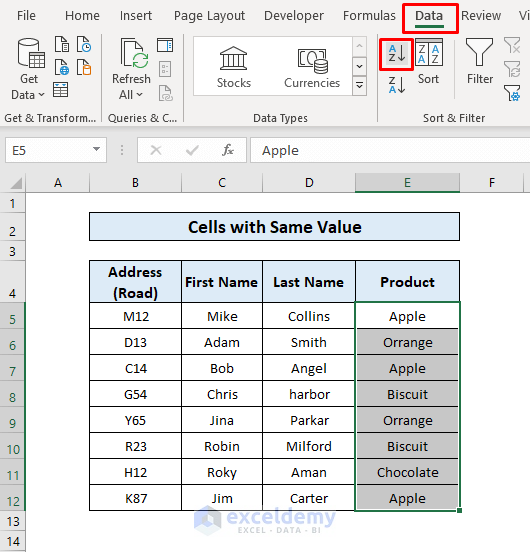
- After sorting, expand the selection to include all relevant cells.
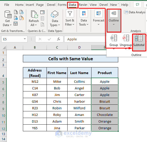
- Go to the Data tab.
- Click the Subtotal button.
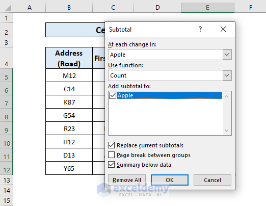
- Specify the text you want to subtotal (e.g., Product).
- Excel will calculate the total number of products based on the grouping.
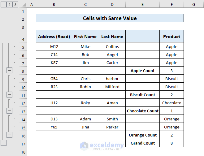
By using the Subtotal feature, we can efficiently group cells with the same value in Excel. This method is especially useful when you need to identify similar values and count the occurrences of repeated items.
Read More: How to Group Duplicates in Excel
Method 3 – Categorize Rows Based on a Similar Text
Suppose you have a dataset in an Excel sheet with a number of similar texts that are slightly different. Your goal is to group these similar texts together. For example, you might have items like Choco Fun 1 and Choco Fun 2 that you want to group.
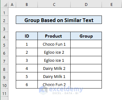
Follow these steps to achieve this:
- In the cell where you want to extract similar texts, use the following formula:
=TRIM(LEFT(SUBSTITUTE(C5," ",REPT(" ",255),2),255))-
- This formula combines several functions:
- TRIM: Removes any unnecessary spaces.
- LEFT: Extracts the name of the product.
- SUBSTITUTE: Replaces numbers from the product items after the second occurrence.
- REPT: Repeats spaces to ensure consistent extraction.
- This formula combines several functions:
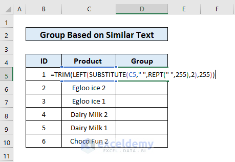
- After entering the formula, press ENTER to get the output in the desired cell.
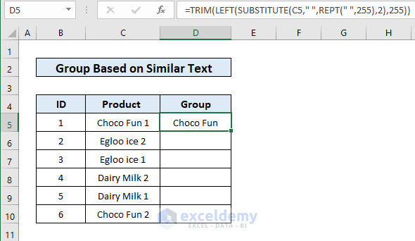
- Drag the formula down to other cells where you want to extract similar texts.
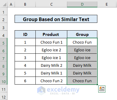
- Once you have the similar texts extracted, go to the Data tab.
- Click Sort A to Z to group the similar texts together.
By following these steps, you can efficiently categorize rows based on similar texts in Excel. This method is especially useful when dealing with nearly identical items that have slight variations.
Method 4 – Grouping Multiple Cells Using Excel’s UNIQUE Function
If you have repeated texts or values in an Excel sheet and you only want the unique texts or values, this method will help you achieve that. Let’s say we have a dataset of products from different countries in a shop, along with their weights. Within this dataset, there are repeated values for certain products, and we want to extract only the unique values.
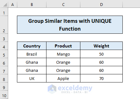
Follow these steps to get the desired result:
- Start by selecting the cell where you want to display the unique value.
- Enter the following formula:
=UNIQUE(B5:B8)-
-
- Here, the UNIQUE function collects the unique names from the specified column (in this case, column B).
-
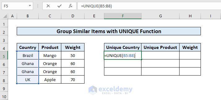
Here, the UNIQUE function collects the unique names from the column.
- After entering the formula, drag it down to apply it to other cells in the same column.
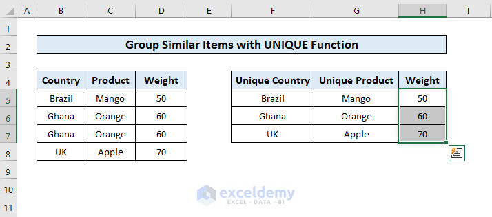
- This will populate the unique values for each corresponding row.
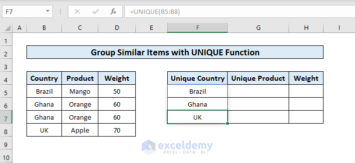
By following these steps, you can easily ignore repeated values and obtain only the unique values you need.
Read More: How to Create Multiple Groups in Excel
Download Practice Workbook
You can download the practice workbook from here:
Related Articles
- How to Remove Grouping in Excel
- How to Use Grouping and Consolidation Tools in Excel
- How to Group Time Intervals in Excel
- How to Group and Ungroup Columns or Rows in Excel
<< Go Back to Group Cells in Excel | Outline in Excel | Learn Excel
Get FREE Advanced Excel Exercises with Solutions!
