Create Home Loan Calculator in Excel Sheet with Prepayment Option

This article shows you how to create a home loan calculator with a prepayment option in an Excel sheet. Using a home loan Excel calculator, you can easily calculate the EMI, monthly interest, remaining principal amount, etc. Here, we will take you through an easy and convenient method on how to create a home loan calculator with a prepayment option in an Excel sheet.

Create Home Loan Calculator in Excel Sheet with Prepayment Option: Step-by-Step Procedure

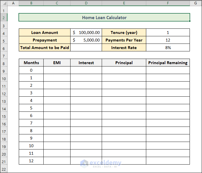
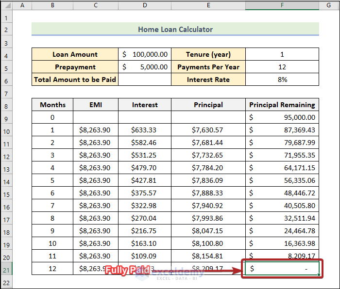
Here, we have created a home loan calculator format. Suppose, we’ve taken a Loan Amount of $1,00,000 for 1-year tenure at an 8% interest rate. The reimbursement system is monthly. For this, we have to repay the loan as EMI. Also, we made a prepayment of $5,000 while taking the loan.

Now, we wanna calculate all these entities in the column header of the blank cells. These are the EMI, Interest, Principal, and the Remaining Principal amount.

Step 1: Calculate the EMI Amount of Home Loan Calculator with Prepayment Option in Excel Sheet

At first, we’ll calculate our EMI amount. Before that, we all should know what EMI actually is. Right? Don’t be panicked if you didn’t know about it earlier. It’s really simple. The EMI, or Equated Monthly Instalment, is one of the equally divided monthly payments that must be settled in order to pay off an outstanding loan within a predetermined period of time.

So, before calculating the EMI, we’ve to make a change in our principal amount. Therefore we don’t wanna apply the EMI over the whole amount of loan we’ve taken. Because we already have made a prepayment to the bank. So, we’ll subtract this prepayment amount from the total loan amount and apply EMI on this.

Firstly, select cell F9 and write down the formula below. Then, hit the ENTER button.

=D4-D5

Here, D4 and D5 represent the cell references of Loan Amount and Prepayment respectively.

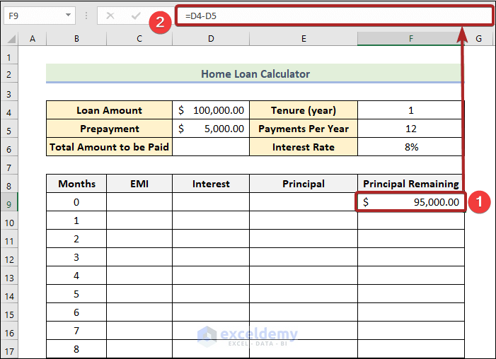
This Principal Remaining amount is at the beginning of the first month. So, the EMI will be calculated based on this amount.

Next, type the formula below in cell C10.
After that, press ENTER.

=PMT($F$6/$F$5,$F$4*$F$5,$F$9)

Here, F6 is the Interest Rate, F5 is the Payments Per Year, F4 is the Tenure and F9 is the Remaining Principal amount. We used the dollar ($) sign for the absolute reference of a cell.

In this formula, we used the PMT function. The PMT is a financial function that determines the loan payment using fixed payments and a fixed interest rate.

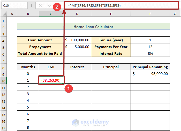
We can clearly see that the output comes as a negative value. Because this amount has to be paid. For our visual convenience, we’ll convert it into a positive value.

Again, select cell C10 and edit the formula like below. Then, press the ENTER key.

=ABS(PMT($F$6/$F$5,$F$4*$F$5,$F$9))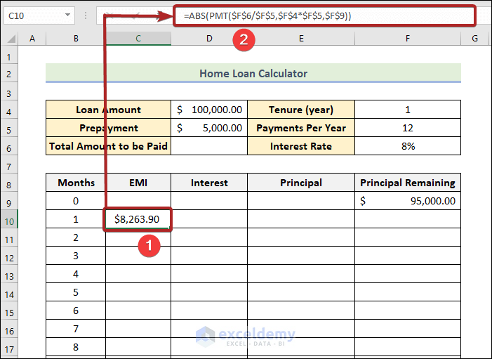

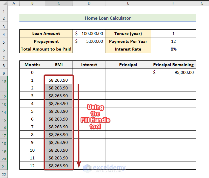
Now, we’ve added the ABS function in front of our previous formula. This function gives a number’s absolute value. The absolute value of a number is its value devoid of its sign.

Hence, easily we can get the EMI amount of our loan.

After that, use the Fill Handle tool and drag it down to cell C21 in order to get the same EMI amount as other months.

Step 2: Count the Interest Per Month

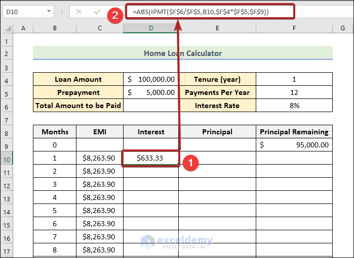
In this step, we’ll calculate the monthly Interest that we have to pay in our EMI.

At first, select cell D10 and put it in the formula below. Then, press ENTER.

=ABS(IPMT($F$6/$F$5,B10,$F$4*$F$5,$F$9))

Here we used the same arguments and cell references as in Step 1. The new thing that hasn’t been used before is the cell reference B10. It denotes the number of Months. For this particular cell, it’s the first month.

Step 3: Work out the Paid-up Capital Per Month

In this phase, we will calculate the monthly paid-up capital.

Firstly, select cell E10 and write down the formula below. Now, press ENTER.

=C10-D10

Simply, subtract the interest from the EMI amount to get the capital amount.

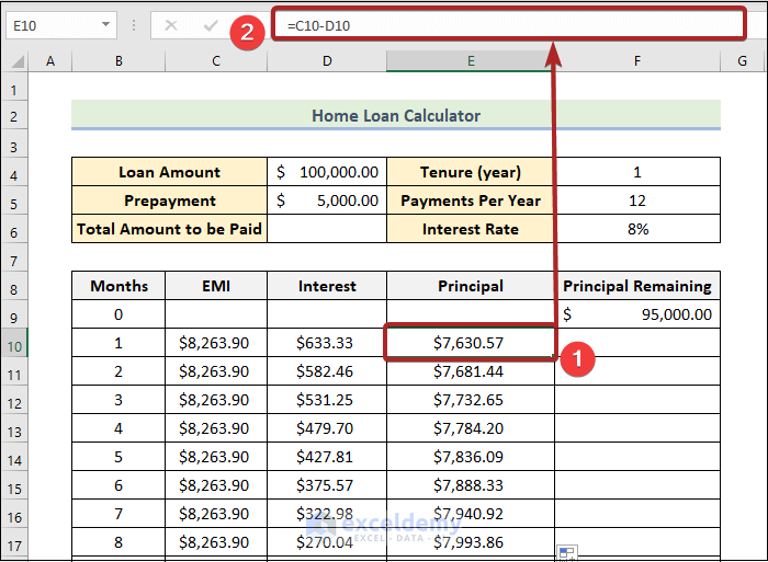
From the above image, we can easily understand visually that the EMI consists of the monthly Interest and the monthly paid-up Principal amount.

Step 4: Determine the Remaining Principal Amount

We also want to calculate the remaining principal amount for each month.

Now, select cell F10. Then, write down the formula below. After that, press the ENTER key.

=F9-E10

Here, F9 and E10 represent the Principal Remaining of last month and the Principal of the present month respectively.

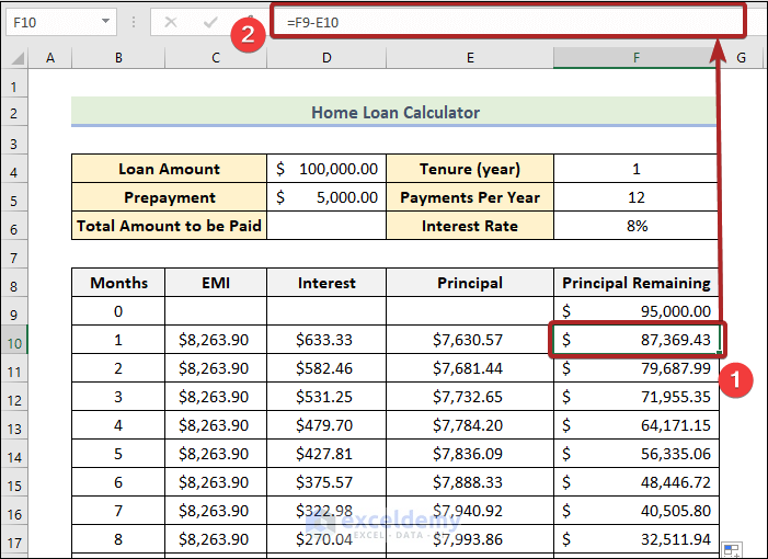
Use the Fill Handle tool and drag it down to cell F21. We can see that our remaining principal amount is showing zero. That means the loan is fully paid in our determined time period of 1 year.

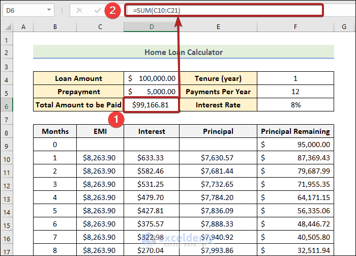
Step 5: Evaluate the Total Amount to be Paid of Home Loan Calculator with Prepayment Option in Excel Sheet

We took a loan of $1,00,000 initially. While taking out the loan, we made a prepayment of $5,000. So, we are bound to pay the EMI of $95,000 in a time period of 12 months.

Finally, select cell D6 and type the formula below. Then, press ENTER.

=SUM(C10:C21)

Here, the SUM function summed up the EMIs in the range C10:C21.

Basically, we have to pay an amount of ( $99,166.81 + $5,000 ) = $104,166.81 while taking a loan of $1,00,000 for a year.

Advantages of Making Prepayment

Prepayment is the early, partial, or complete repayment of a debt by the borrower. There are several advantages of prepayment. We can easily notice this below.

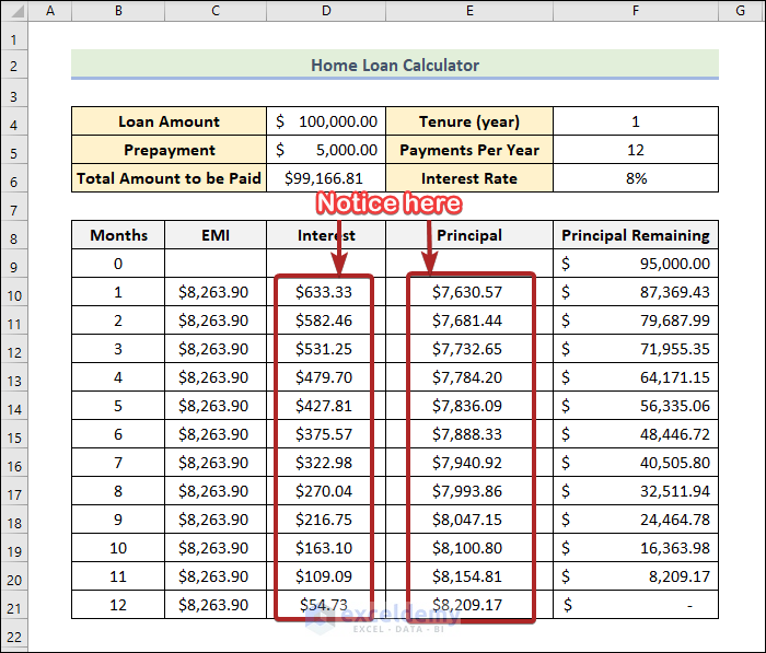
From the image above, we can definitely observe that the monthly Interest is gradually decreasing. As a result, the monthly paid-up Principal is increasing continuously. Because our EMI is constant over the period of 12 months. So, if we can make a handsome amount of prepayment in the beginning, the burden of interest will be less upon us.

Without making any kind of prepayment, our loan status would be like the image below.

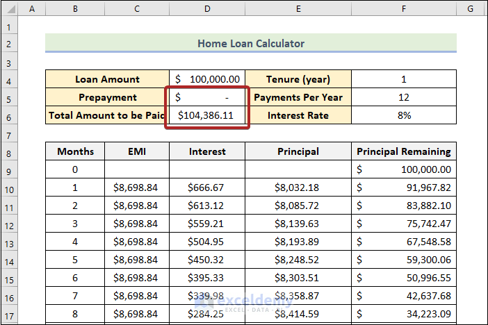
Easily, we can detect that the Total Amount to be Paid here is greater than that of the $5,000 Prepayment.

Download Practice Workbook

You may download the following Excel workbook for better understanding and practice yourself.

Home Loan Calculator with Prepayment Option.xlsx

Conclusion

Thank you for reading this article, we hope this was helpful. Please let us know in the comment section if you have any queries or suggestions. Please visit our website to explore more.

<< Go Back to Loan Calculator | Finance Template | Excel Templates

Get FREE Advanced Excel Exercises with Solutions!