How to Calculate Accumulated Depreciation in Excel: 9 Easy Ways

Method 1 – Apply Simple Depreciation Formula

Steps:

• Click on the left button of the mouse to select empty cell D5.
• Write down the following formula in the formula bar.

• $D$15 refers to the value of cell D15, $D$16 refers to the value of cell D16 and $D$17 is an absolute reference to cell D17.

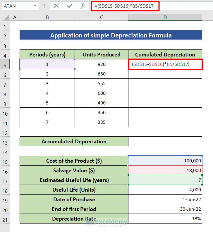
• Press the Enter button to see the cumulative depreciation of the period of year 1.

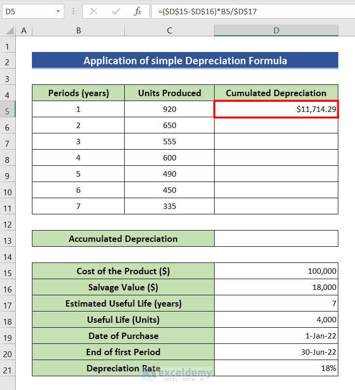
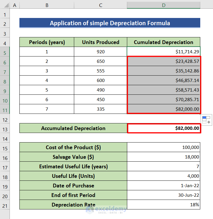
• To get the cumulative depreciation value for periods 2 to 7 years, double-click the bottom right corner of cell D5.
• Cell D11 and D13 will show the cumulative depreciation of the 7-year period which is also the accumulated depreciation.

Method 2 – Use the Units of Production Formula

Steps:

• Bring your cursor to cell D5 and click on it.
• Type the following formula in that cell.

• In this formula, $D$15, $D$16, $D$18 are absolute references to cells D15, D16, and D18, and C5 refers to the value of cell C5.

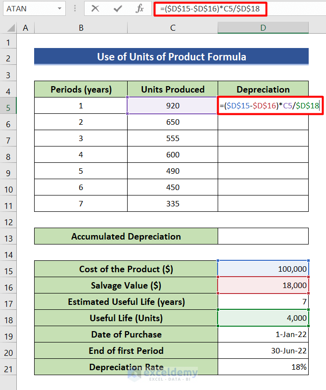
• Hit Enter. Depreciation of the 1st period will be shown in cell D5.

• Drag the bottom right corner of cell D5 to cell D11.

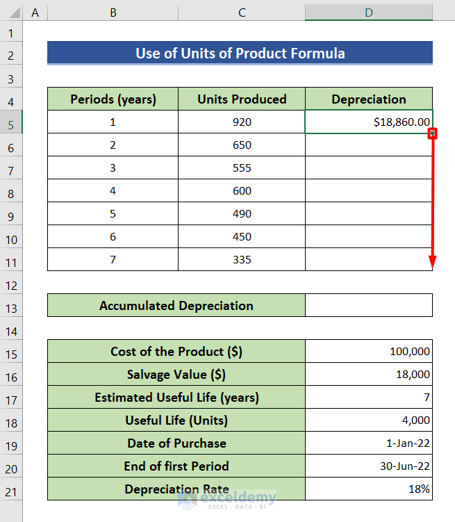
• Get the results for all 7 years.

• Find the value of accumulated depreciation, go to cell D13 and write down the following formula.

• D5:D11 refers to all cell values from D5 to D11.

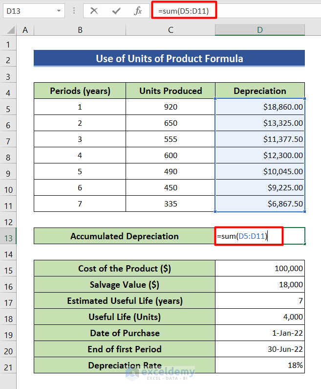
• The SUM function will add up all the depreciation of 7 years and give the accumulated depreciation.

Method 3 – Insert SYD Function

Steps:

• Select cell D5 and write down the formula given below.

• $D$15, $D$16, $D$17 are absolute references to cells D15, D16 and D18 respectively and B5 refers to cell B5.

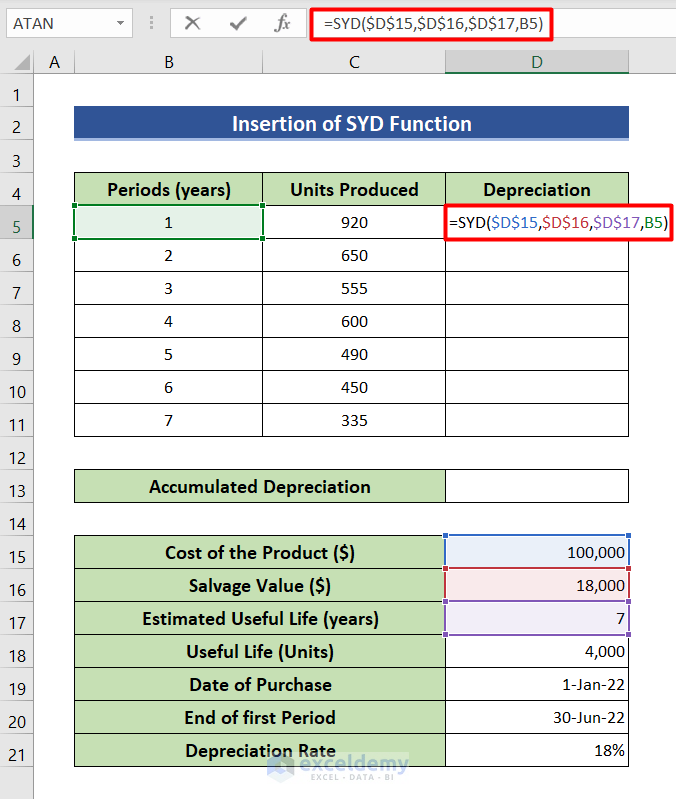
• Hit the Enter button to see the depreciation in cell D5.

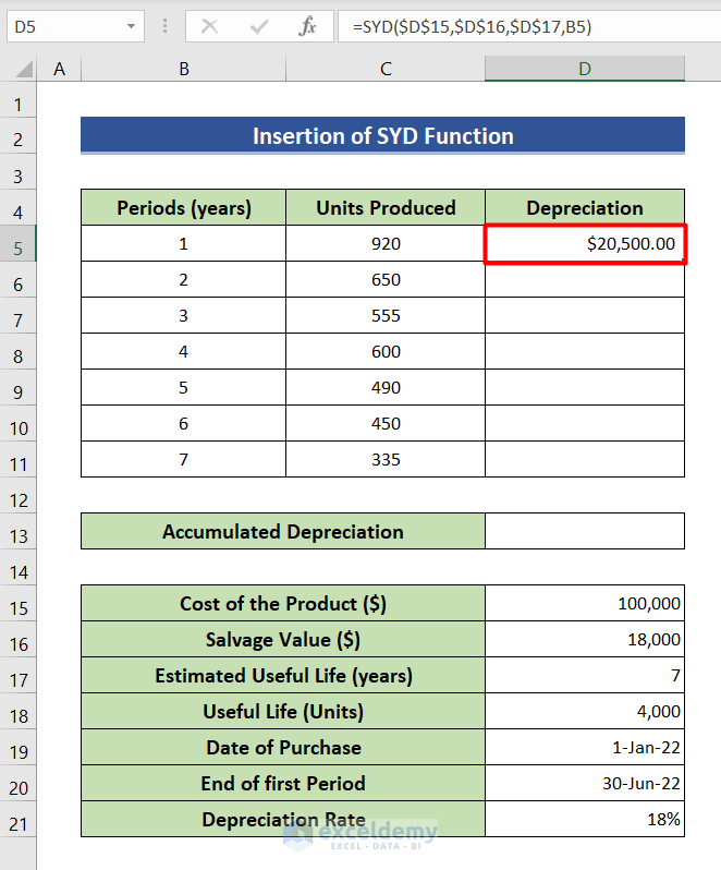
• Double-click on the bottom right corner of cell D5 to get the depreciation value for all data.

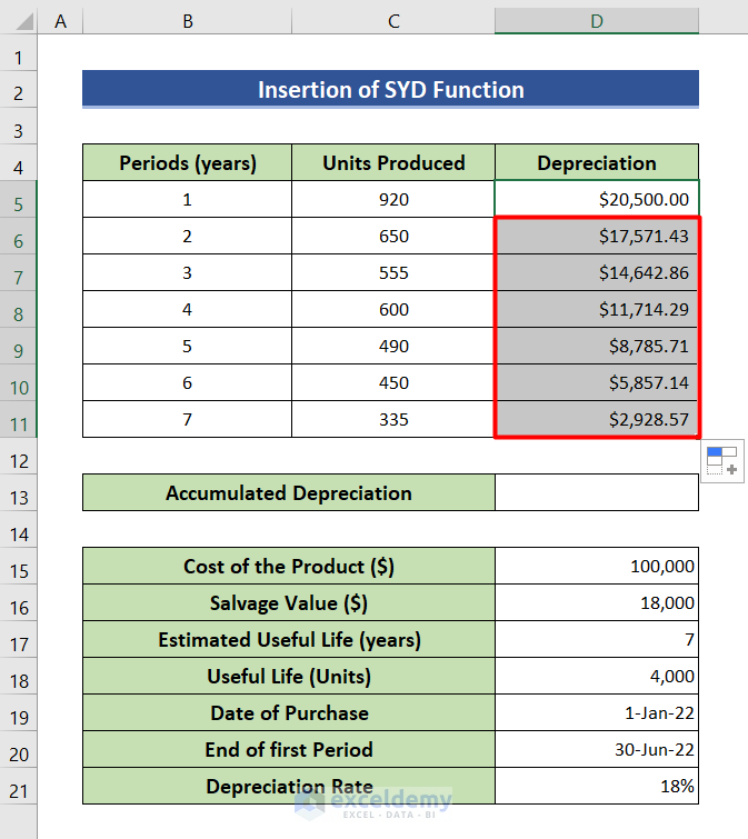
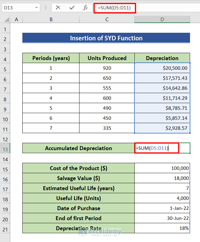
• See how to determine the accumulated depreciation from all the depreciation values. Type the sum formula in cell D13.

• D5:D11 refers to cells D5 through D11.

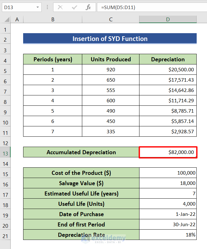
• If you press Enter, you will get the accumulated depreciation in cell D13.

Method 4 – Apply Straight-Line Method

Steps:

• Uuse your mouse to select D5.
• Now you need to type the SLN formula in that cell.

• $D$15 refers to the value of cell D15, $D$16 refers to the value of cell D16 and $D$17 is an absolute reference to cell D17.

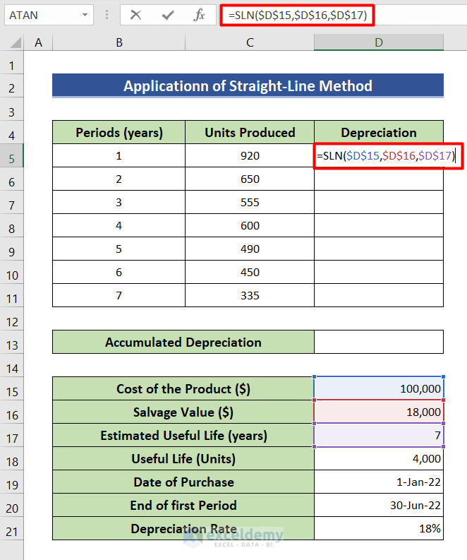
• To get the result in cell D5, press Enter.

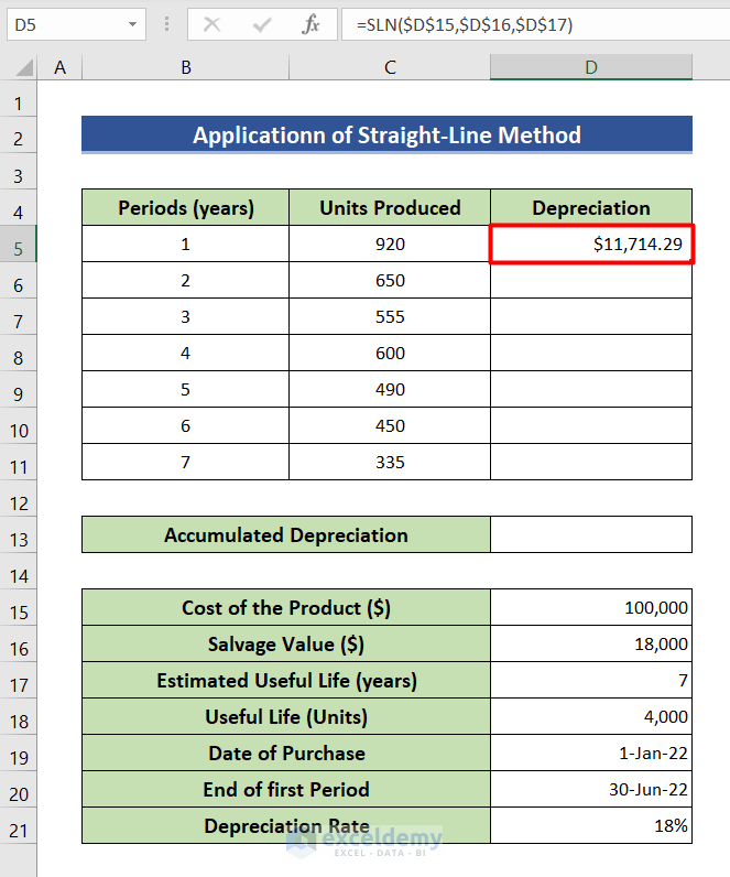
• Bring your cursor to the bottom right corner of cell D5 and click the left button of the mouse two times.
• This will give you depreciation value for periods 2 through 7.

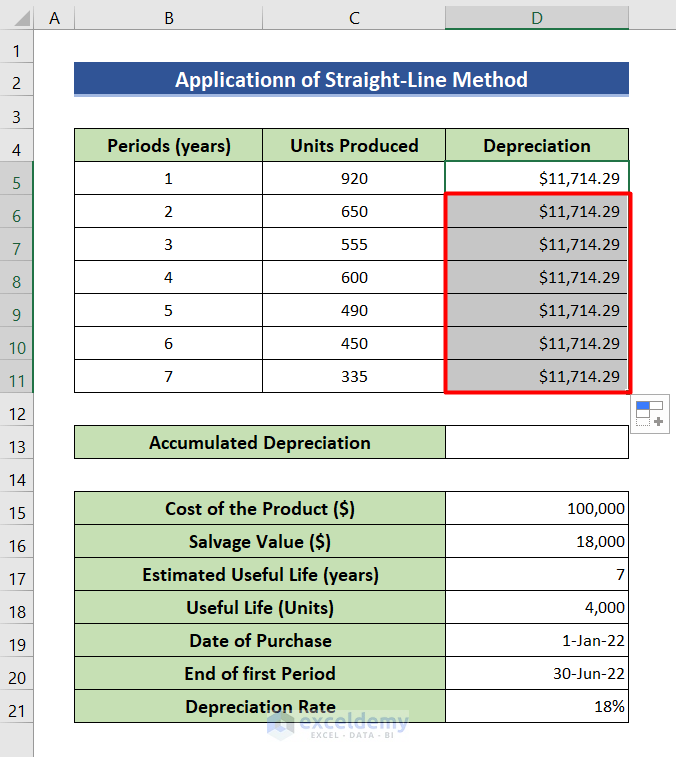
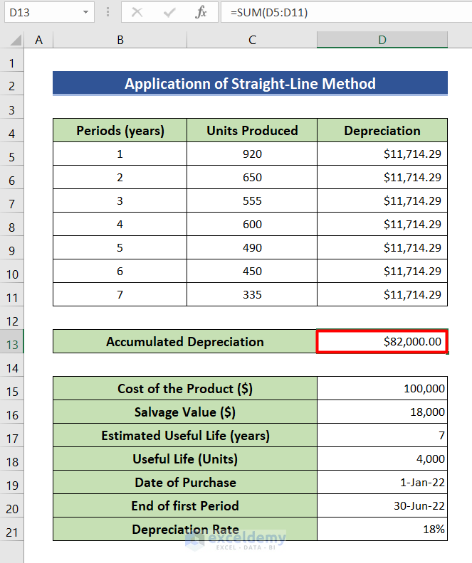
• Use the SUM function to determine the accumulated depreciation. Use the following formula, where D5:D11 refers to the depreciation of cells D5 to D11.

• Hit Enter and see the desired accumulated depreciation value.

Method 5 – Utilize VDB Function

Steps:

• Go to cell D5 and click on it.
• Write down the following formula in the formula bar.

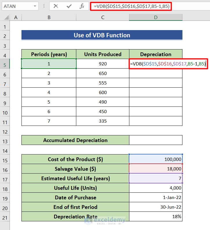
• Hit Enter on the keyboard to find out the depreciation of 1st year.

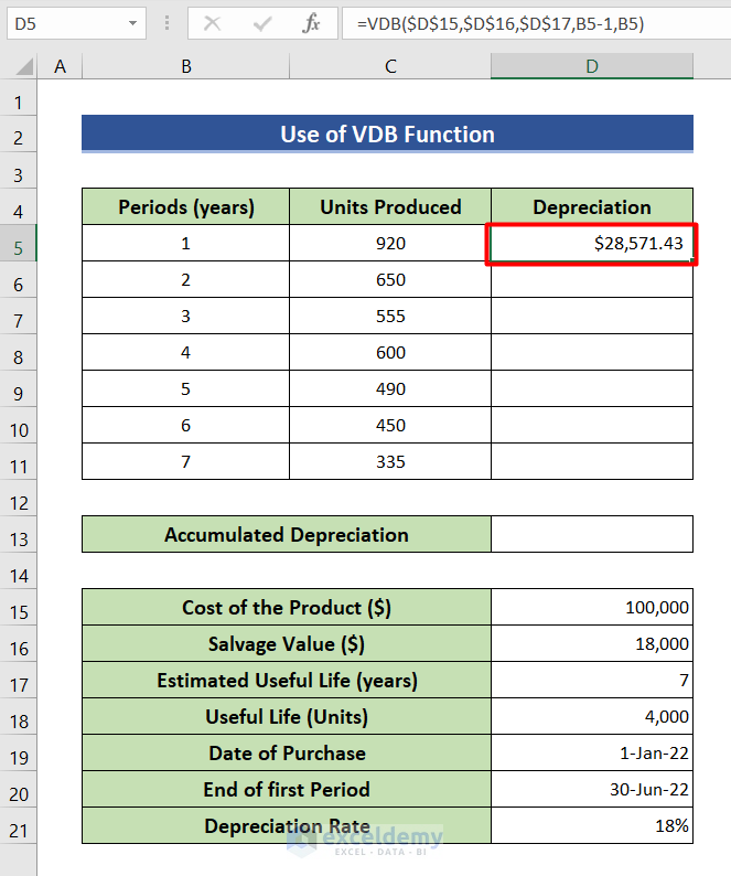
• Double-click the bottom right corner of cell D5. This will give you depreciation for the whole period.

• Use the following sum formula to calculate accumulated depreciation.

• D5:D11 refers to all the values of D5 to D11.

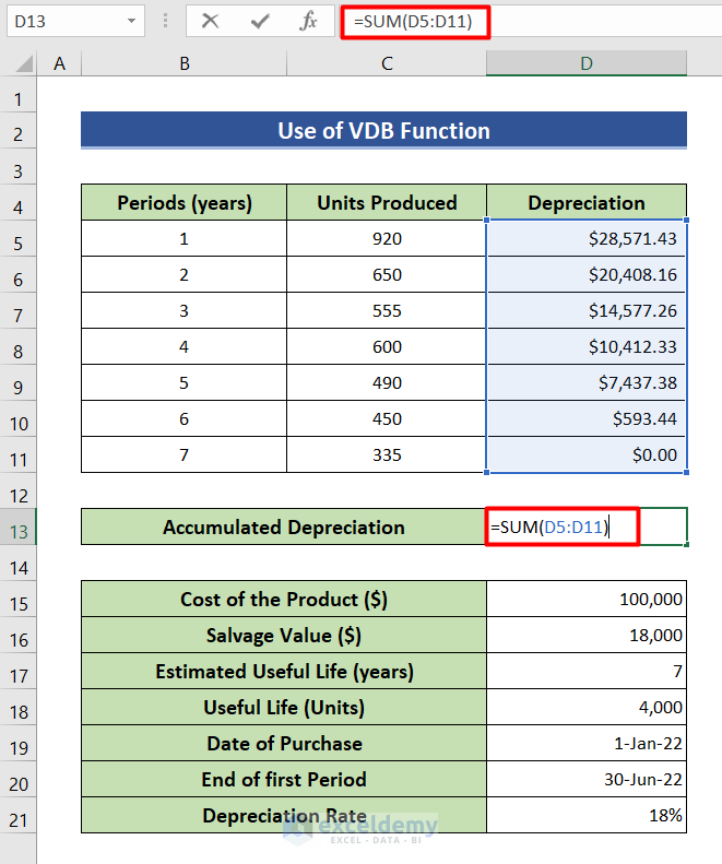
• Press Enter and get the accumulated depreciation.

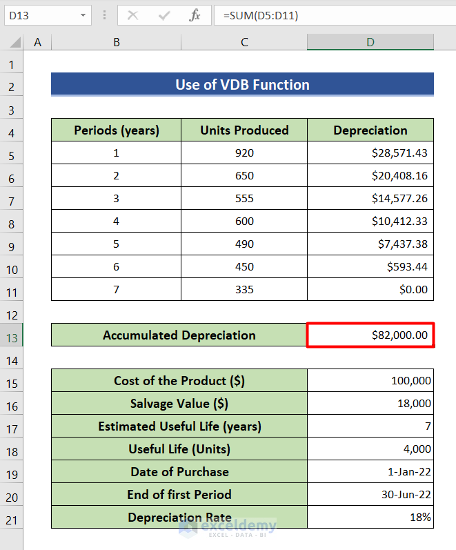
Method 6 – Use DB Function

Steps:

• Select cell D5 and type the below formula.

• $D$15, $D$16, $D$17 are absolute references to cells D15, D16 and D17 respectively and B5 refers to the value of cell B5.

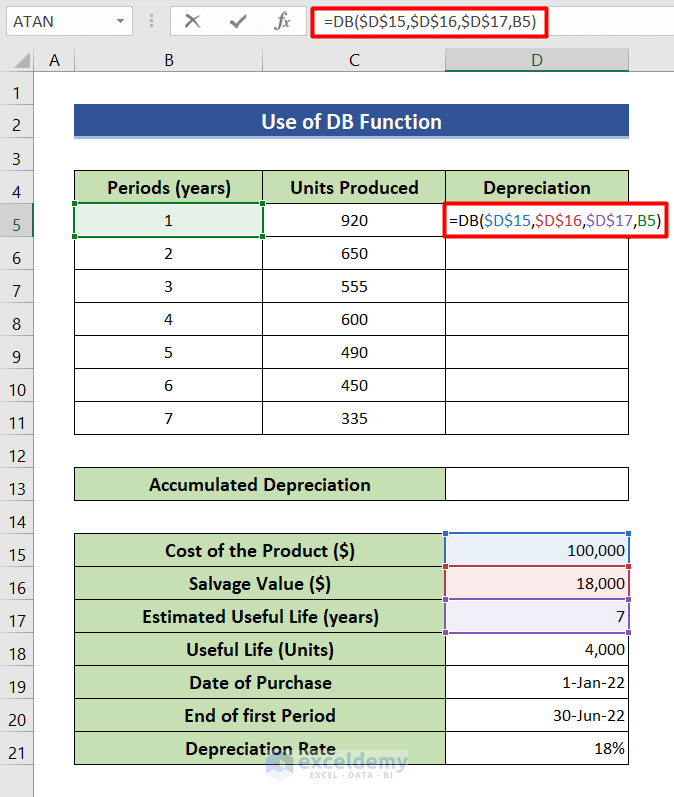
• Hit Enter and get the result in cell D5.

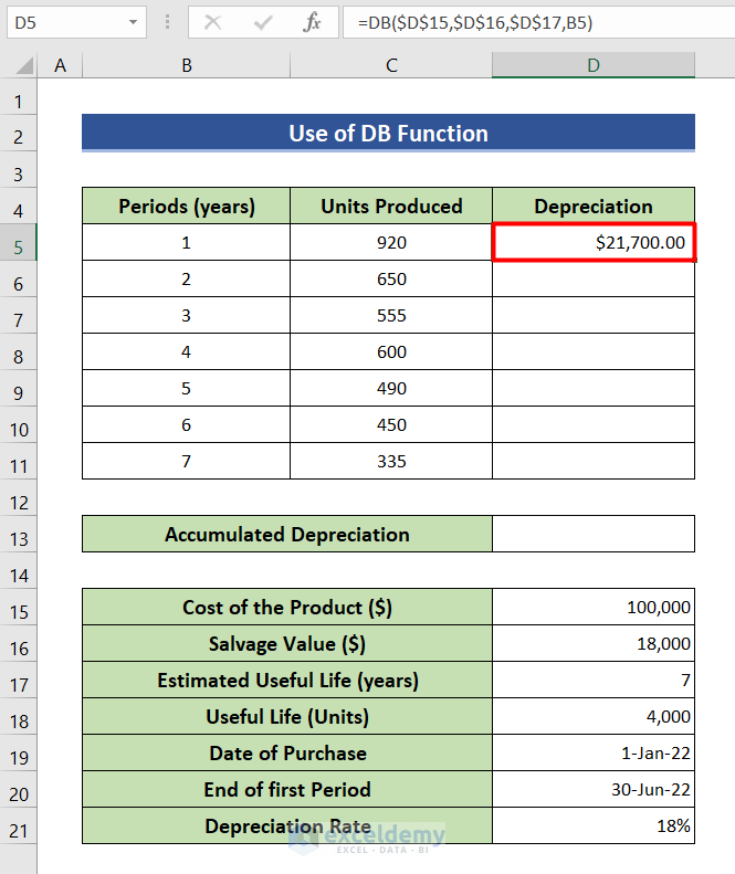
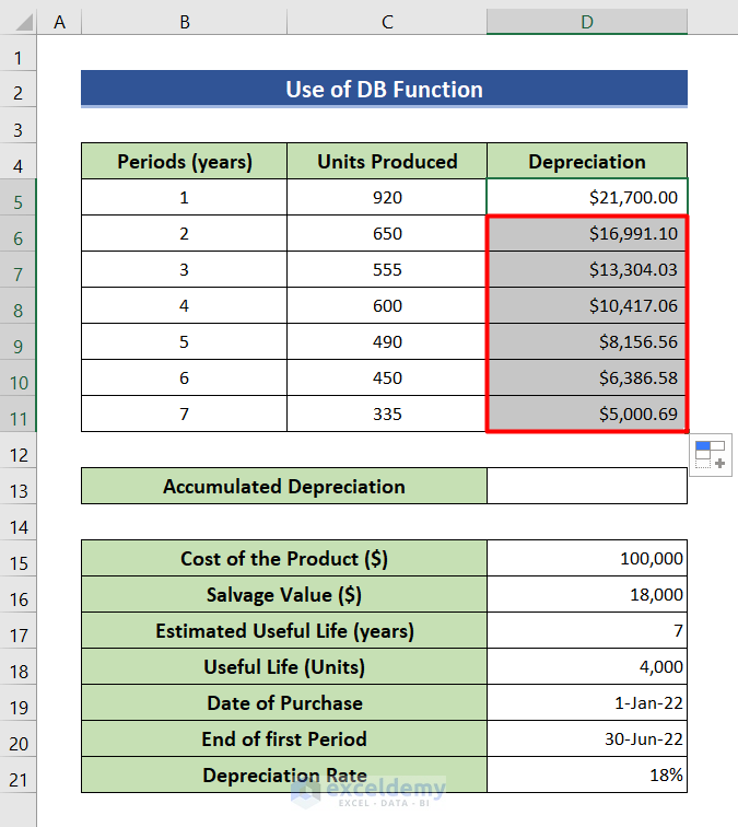
• Move your cursor to the bottom right corner of cell D5 and double-click on it.
• This will show the results for all 7 years.

• Use the following formula to get the accumulated depreciation.

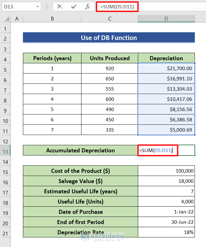
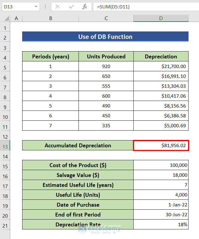
• Press Enter on the keyboard. It will sum up all the depreciation and give the accumulated depreciation.

Method 7 – Apply DDB Function

Steps:

• Click on cell D5 and write down the following formula.

• $D$15, $D$16, $D$17 are absolute references to cells D15, D16, D17 and B5 refers to the value of cell CB5.

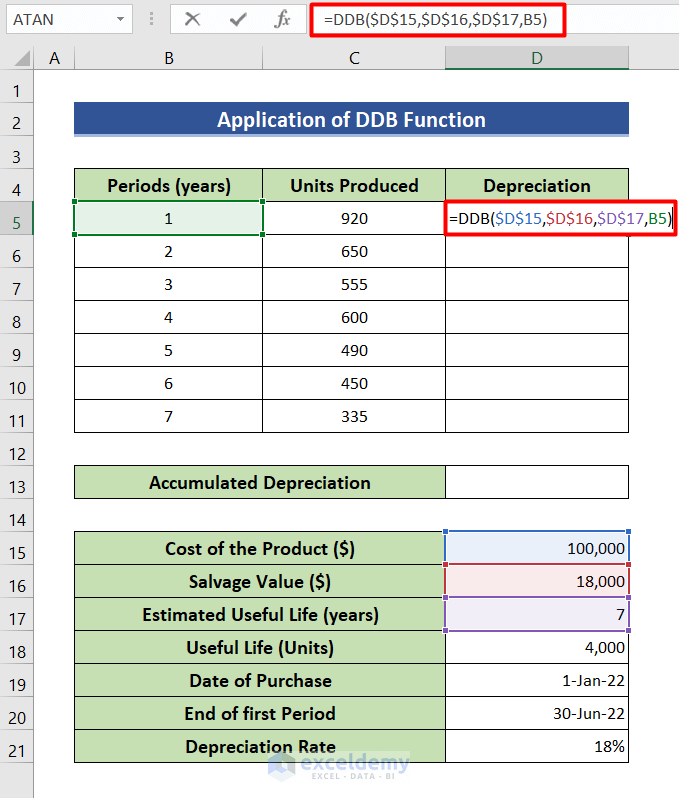
• Hit Enter.
• It will give you the result of the 1st period.

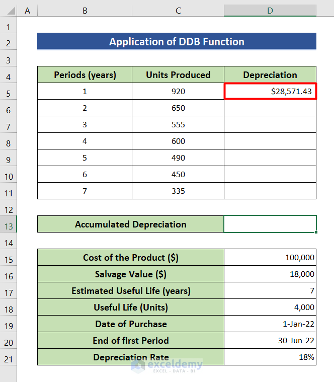
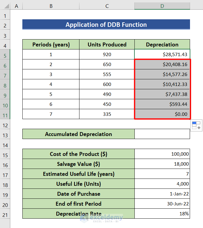
• To find out the depreciation over the full 7 years, double-click the bottom right corner of cell D5.

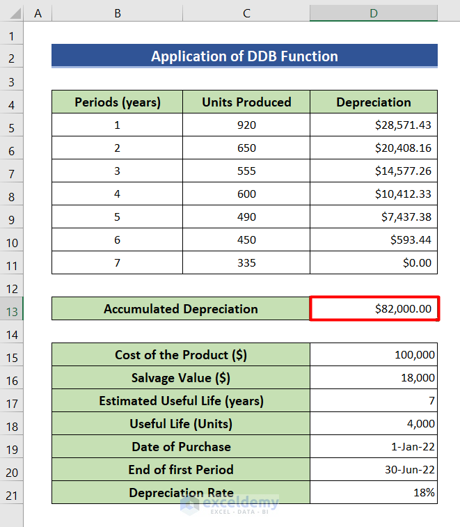
• Write the following sum formula to get the accumulated depreciation.

• It will add up all the values from D5 to D11 and give the desired result.

Method 8 – Insert AMORLINC Function

Steps:

• Type the following formula in cell D5.

• In this formula, $D$16,$D$20,$D$21,$D$17 refers to cells D16, D20, D21 and D17 B5 refers to the value of cell B5 and $D$22 is absolute reference to cell D22.

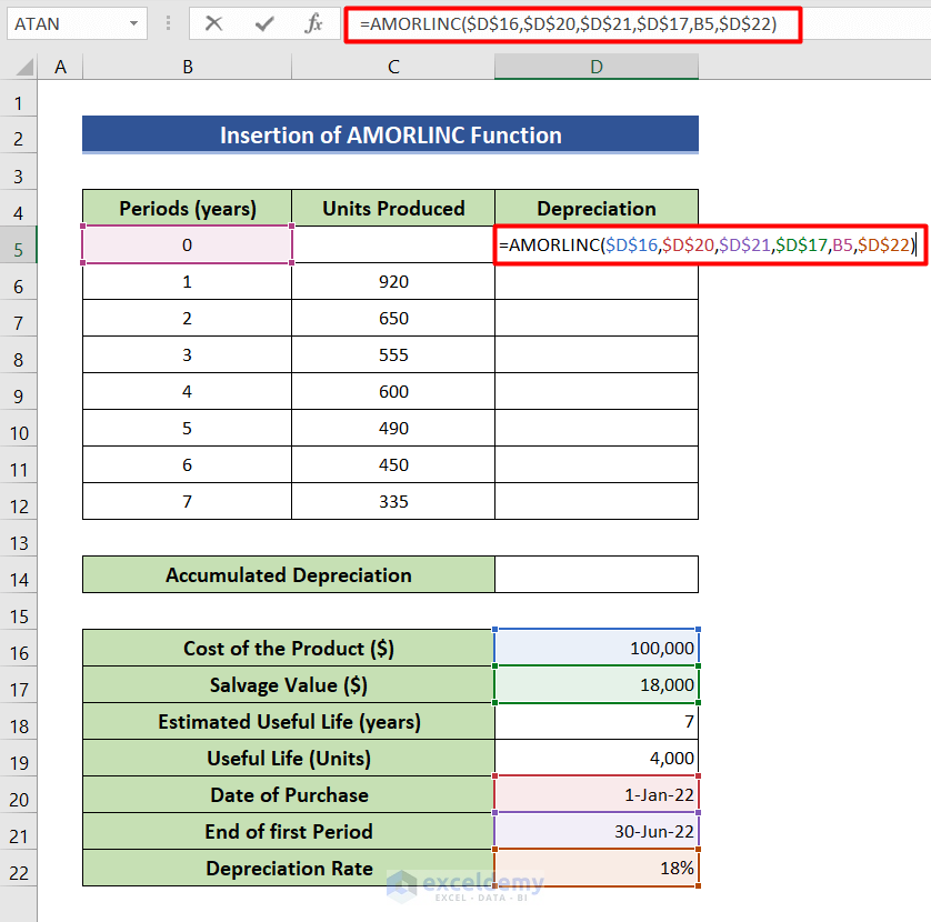
• Press the Enter button and find the result in cell D5.

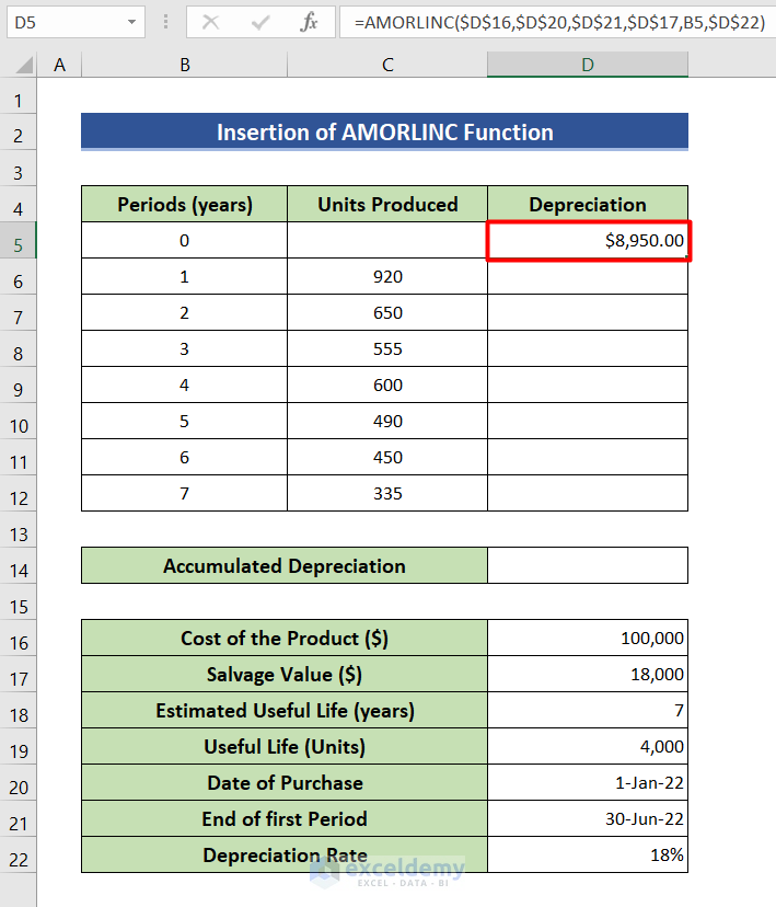
• Double-click the bottom right corner of cell D5 to get results for the whole period.

• Find out the accumulated depreciation, use the sum formula, where D5:D12 refers to cells D5 through D12.

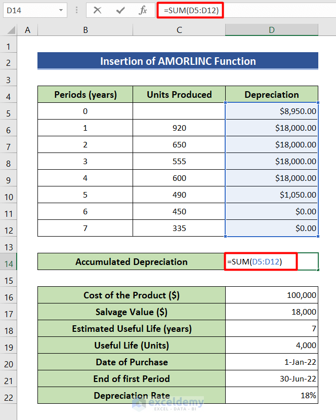
• Hit Enter and see the desired accumulated depreciation.

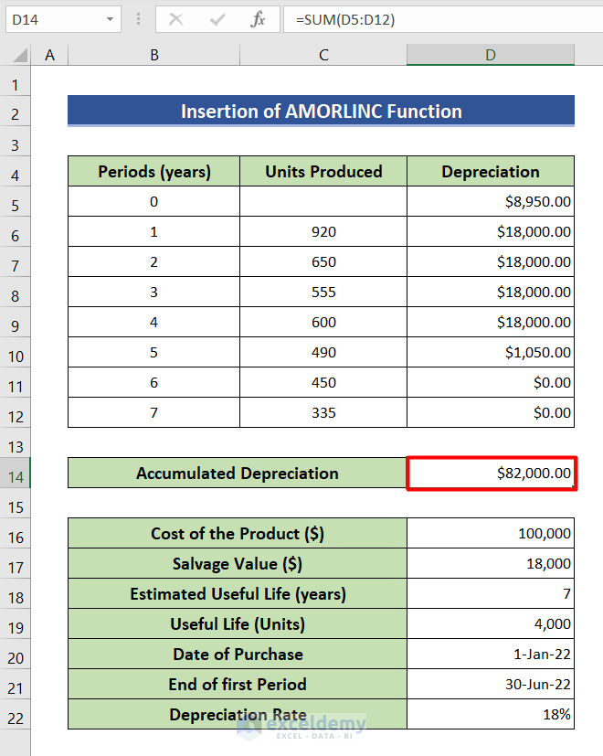
Method 9 – Use AMORDEGRC Function

Steps:

• Select empty cell D5.
• Write down the AMORDEGRC formula.

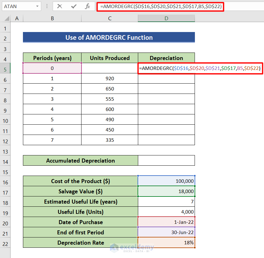
• To get the result for the 1st year, hit Enter.

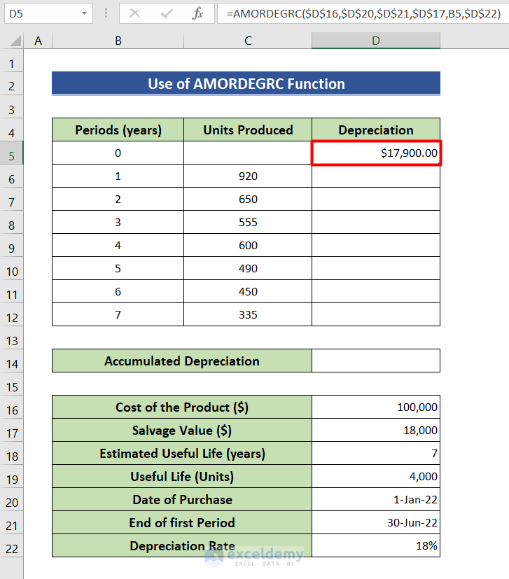
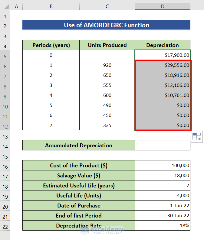
• Double-click the bottom right corner of cell D5.
• This gives you all the depreciation value.

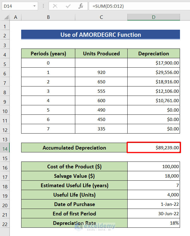
• Find the accumulated depreciation. Use the SUM function, where D5:D12 refers to cells D5 to D12.

• Press Enter and get the accumulated depreciation.

Things to Remember

• While using a formula, don’t forget to give proper cell references or you won’t get the desired results.
• Use the absolute reference sign ($) for the formulas otherwise, you can get erroneous results.

Download Practice Workbook

Download this practice workbook for practice while you are reading this article.

Related Articles

• How to Use WDV Method of Depreciation Formula in Excel
• How to Use MACRS Depreciation Formula in Excel
• How to Use Formula to Calculate Car Depreciation in Excel
• How to Calculate Double Declining Depreciation in Excel

<< Go Back to Depreciation Formula In Excel|Excel Formulas for Finance|Excel for Finance|Learn Excel