Method 1 – Combine DATEDIF, TODAY, and AVERAGE Functions to Calculate Average Tenure of Employees
1.1 Dynamic Date
Steps:
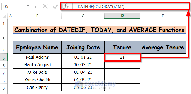
- Select cell D5, and write down the below formula.
=DATEDIF(C5,TODAY(),"M")Formula Breakdown:
- Inside the DATEDIF function, C5 is the start_date, TODAY is the end_date, and M is the format of the DATEDIF function.
- Since we want to see the result on the current day, it’s ideal to calculate using the TODAY function. If you use the TODAY function, when you open this workbook for a couple of days/months (whenever you like), it will show the result based on that day.
- We put M to get the difference in months.
- Press Enter on your keyboard. Get the tenure which is the return of the DATEDIF function. The return is 21.
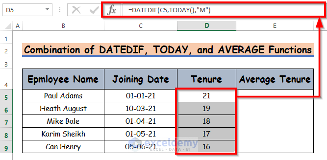
- Autofill the functions to the rest of the cells in column D.
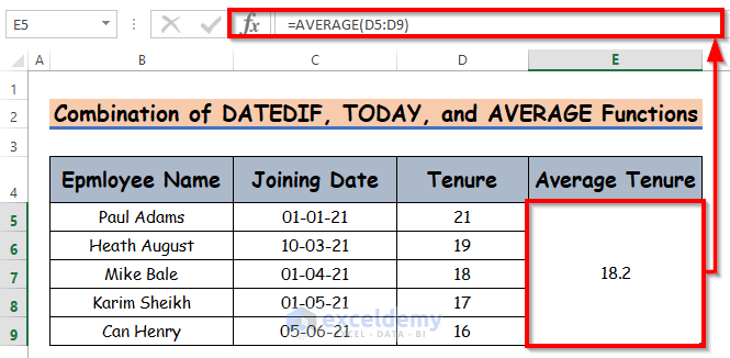
- Calculate the average tenure now. To calculate the average tenure, write the AVERAGE function in cell E5.
=AVERAGE(D5:D9)- Press Enter on your keyboard. Get the tenure which is the return of the AVERAGE function. The return is 2.
- Within the AVERAGE function insert the range of your calculated tenure for each employee, it will give you average tenure.
- We showed the difference in months. Get the output in years as well. Just use Y instead of M.
In the above sub-method, you can also use the NOW function instead of the TODAY function. The result will remain the same.
1.2 Specific Date
Steps:
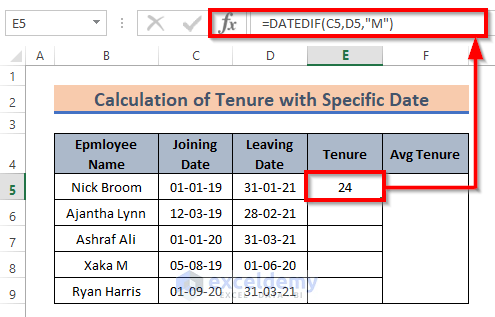
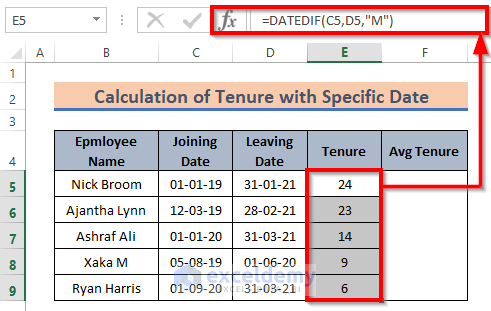
- Select cell E5, and write down the below.
=DATEDIF(C5,D5,"M")- Press Enter on your keyboard.Get the tenure which is the return of the DATEDIF function. The return is 24.
- AutoFill the functions to the rest of the cells in column E.
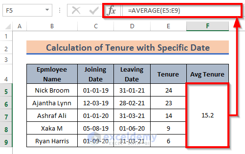
- Calculate the average tenure, write the AVERAGE function in cell E5.
=AVERAGE(E5:E9)- Press Enter on your keyboard. Get the tenure which is the return of the AVERAGE function. The return is 2.
- Here we got the result in monthly format.
Method 2 – Applying DATEDIF Function to Calculate Tenure in Year-Months Format
Steps:
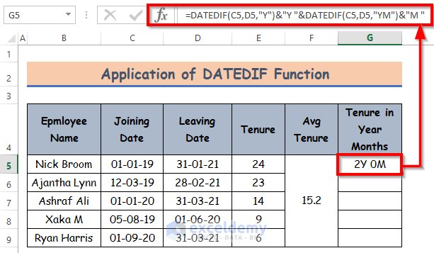
- Write the DATEDIF formula in cell G5.
=DATEDIF(C5,D5,"Y")&"Y "&DATEDIF(C5,D5,"YM")&"M "- Press Enter on your keyboard. Get the tenure in year and month format which is the return of the DATEDIF function. The return is 2Y 0M.
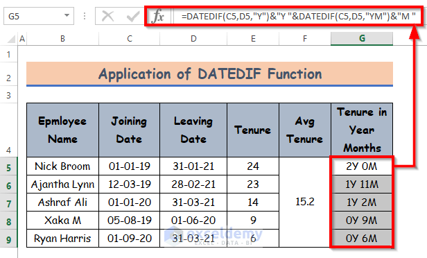
- AutoFill the functions to the rest of the cells in column D.
- We inserted Joining Date and Leaving Date in the placeholders for start_date and end_date and concatenated Y and M to the outside of the DATEDIF function so that the result would be presented with a unit.
Employees Tenure Calculator
You can use today’s workbook as a calculator to count average employees’ tenure. There is a sheet named Calculator.
Explore that sheet. You will find fields for the Joining Date, and Leaving Date. Insert your values. It will calculate Tenure and the Average Tenure which has been given in the below screenshot.
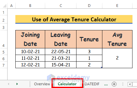
For your understanding purpose, we gave an example with the values of three employees. You can insert as many employees as you want.
Download Practice Workbook
You can download the practice workbook from the link below.
Further Readings
- How to Calculate Overdue Days in Excel
- How to Calculate Remaining Days in Excel
- How to Calculate Working Capital Days in Excel
- How to Calculate Days Outstanding in Excel
- How to Calculate 90 Days from a Specific Date in Excel
- How to Create a Day Countdown in Excel
<< Go Back to Days Between Dates | Date-Time in Excel | Learn Excel
Get FREE Advanced Excel Exercises with Solutions!

