In the dataset, you will see the profit data of a company for 4 years. The last one is the target profit (profit data in 2021). To achieve this, we will calculate what the CAGR value should be.
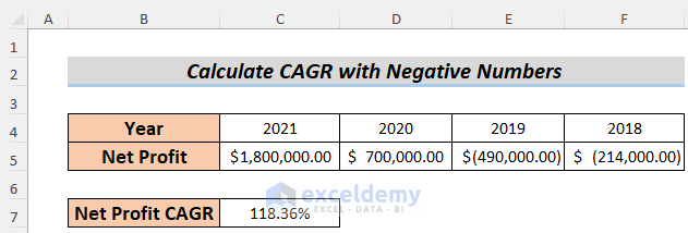
The mathematical formula to calculate the CAGR is given below.

Read More: How to Calculate End Value from CAGR in Excel
Method 1 – Using Excel ABS Function to Calculate CAGR with Negative Number
As the fractional root of a negative number returns complex values, we will use the ABS functions to calculate the absolute values of negative profit (loss in business) to calculate the CAGR.
Steps:
- Insert the data of profit over the years.
- Copy the following formula in the cell:
=((C5-F5+ABS(F5))/ABS(F5))^(1/(C4-F4))-1
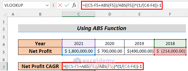
The formula is derived from the CAGR formula we showed in the previous section. The ABS function makes the loss value positive and thus removes the complex number dilemma.
- Press the Enter button and you will see the CAGR value for the data we use in this sheet.
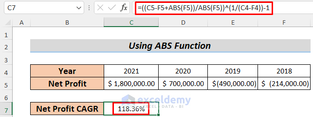
Thus you can calculate the CAGR by using the Excel ABS function with negative numbers.
Read More: How to Calculate Future Value When CAGR Is Known in Excel
Method 2 – Applying Goal Seek Analysis to Calculate CAGR with a Negative Number
Steps:
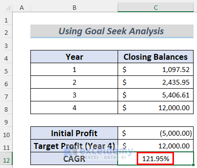
- Set the initial profit and target profit. Choose a CAGR of your choice. As our topic focuses on negative numbers, we are considering that the company made a loss in the first year.
- Copy the following formula in cell C5.
=C10+ABS(C10)*$C$12
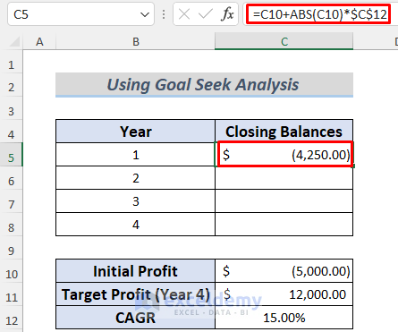
The formula will return the principal after a year with a CAGR of 15% referenced by cell C12. Note that we are using the ABS function to get rid of negative values.
- Copy a similar formula in cell C6:
=C5+ABS(C5)*$C$12
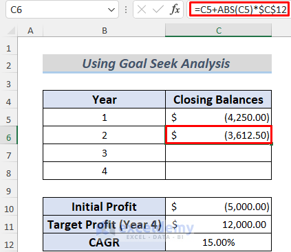
This formula also returns the principal in the second year.
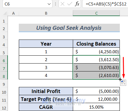
- Select C5 and C6.
- Use the Fill Handle to AutoFill the lower cells.
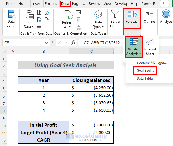
- Go to Data, select Forecast, choose What if Analysis, and pick Goal Seek.
- Select C8 as the Set Cell. Because we want to find out the CAGR by making the value of this cell to our target value (12000).
- The ‘To Value’ will be 12000.
- The CAGR is in cell C12 so we selected it for the ‘By Changing Cell’ section.
- Click OK.
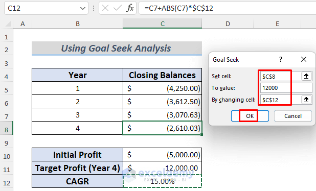
- This operation will provide you with the CAGR based on this dataset.
Read More: Excel Formula to Calculate Average Annual Compound Growth Rate
Practice Section
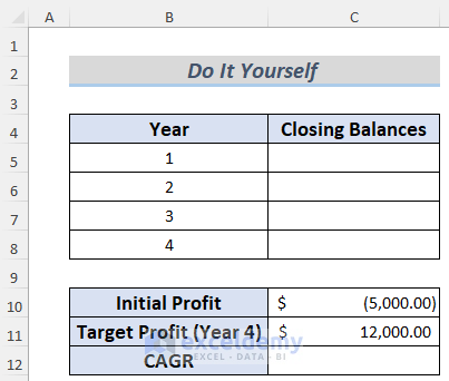
Here’s the dataset of this article so that you can practice these methods on your own.
Download Practice Workbook
Related Articles
- How to Calculate 3-Year CAGR with Formula in Excel
- How to Calculate 5 Year CAGR Using Excel Formula
- How to Create CAGR Graph in Excel
<< Go Back to Compound Interest in Excel | Excel for Finance | Learn Excel
Get FREE Advanced Excel Exercises with Solutions!

