Formula to Calculate Kurtosis
Despite having a biased estimation if you do not have the full-scale data of a given phenomenon, we will calculate the Kurtosis using the Population Kurtosis Formula in this article. It is denoted mathematically by the following formula:
Kurtosis =Fourth Moment value/Square of second Moment valueWhere,

and,

Here,
- n= Sample size
- Xi= sample value
- Xavaerage= mean value of the sample values.
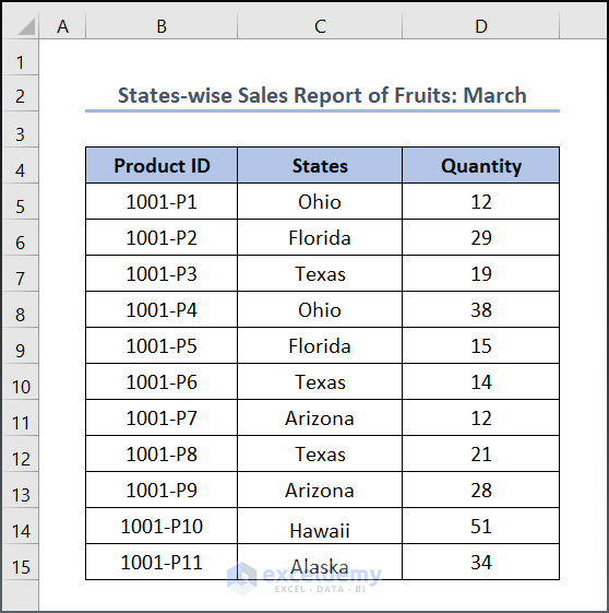
We take into account a random variable x and a data collection of size n, S = {x1, x2,…, xn} that contains all possible x values. The dataset may reflect the entire population under study or a sample from it. Below is our dataset, “States-wise Sales Report of Fruits: March”.
Method 1 – Applying an Arithmetic Formula
Steps:
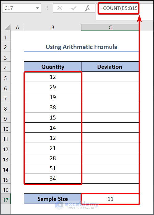
- Enter the following formula in the C17 cell:
=COUNT(B5:B15)
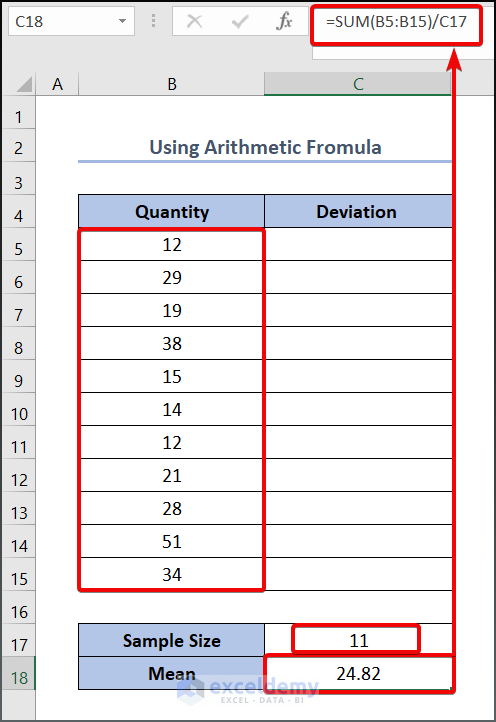
- To calculate the mean value,
- Enter the following formula in cell C18:
=COUNT(B5:B15)
Here, B5:B15 refers to the numerical values of each data and C17 represents the sample size.
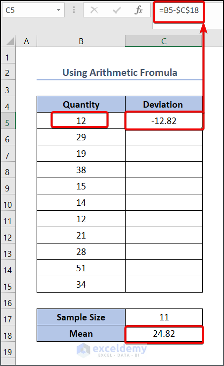
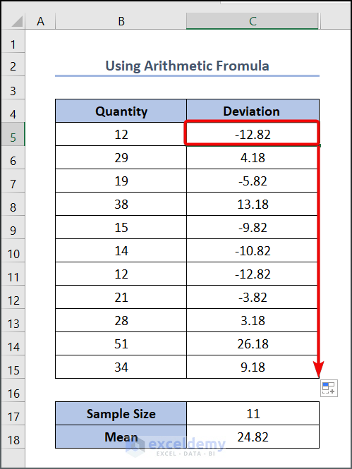
- To calculate the deviation of each value from the mean value,
- Enter the following formula in cell C5:
=B5-$C$18
We have locked cell C18 because we have to use it to get the other value.
- Drag the Fill Handle tool to get the other values.
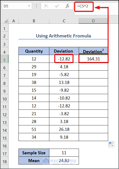
- Enter the following formula in cell D5 to calculate the squared value of the deviation.
=C5^2
- Press OK to see the output.
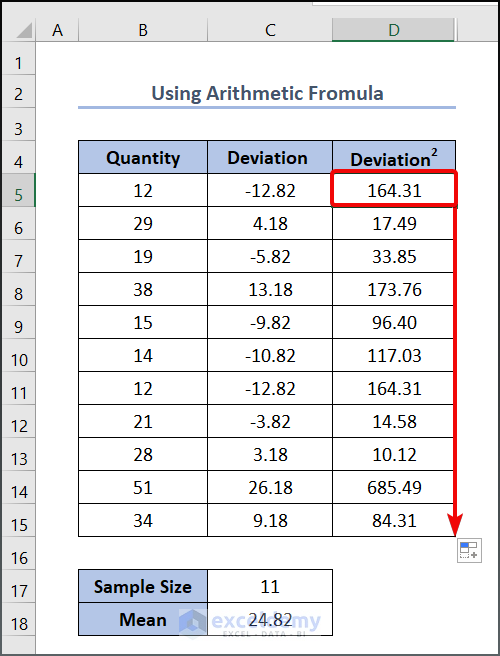
- Drag the Fill Handle tool to get the other values.
- Enter the following formula in cell E5:
=C5^4
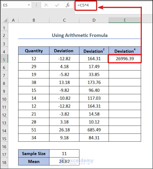
- Lower the cursor to cell E15 to use the AutoFill tool.
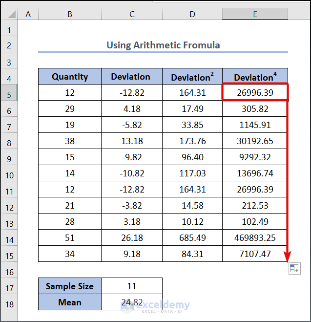
- To calculate the second moment,
- Enter the following formula in cell E17:
=SUM(D5:D15)/C17
- Press the Enter button to see the output below.
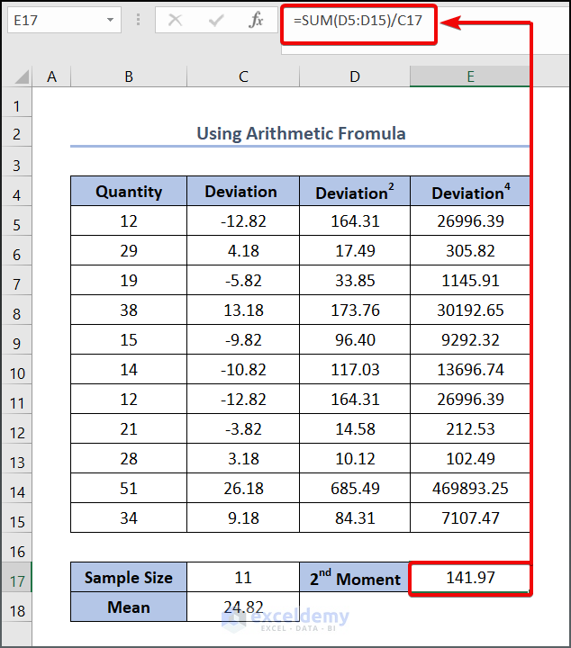
- To calculate the fourth moment,
- Enter the formula in cell E18:
=SUM(E5:E15)/C17
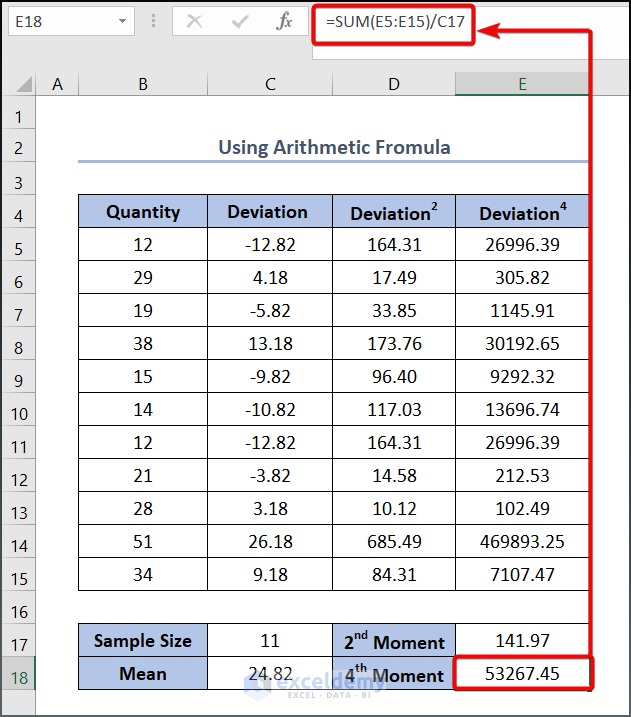
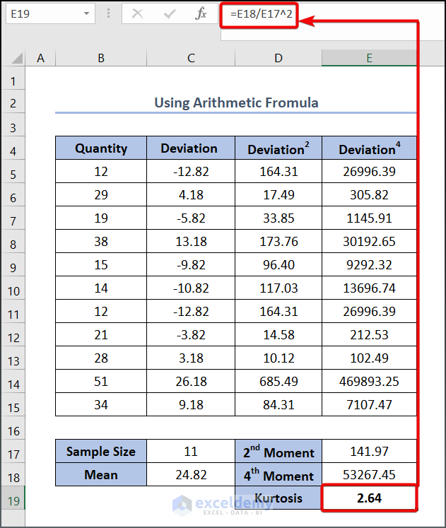
- Enter the following formula in cell E19:
=E18/E17^2
Here, E17 refers to the second-moment value, and E18 refers to the fourth-moment value.
- Press Enter to see the output as below.
Read More: How to Calculate Skewness in Excel
Method 2 – Using the KURT Function
Steps:
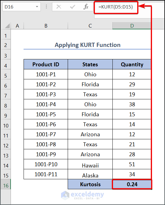
- Enter the following function in cell D16:
=KURT(D5:D15)
- Press the Enter key to see the output.
Read More: How to Calculate Coefficient of Skewness in Excel
Things to Remember
- The maximum argument the KURT function can hold is 30. If your dataset is larger than 30, you will face trouble using this function.
- Similarly, the minimum number of arguments to get the output from the KURT function is 4. So if your sample size is less than 4, then an error will occur. To avoid such a situation, input a value, even zero, as your argument to fulfill the minimum requirement.
Practice Section
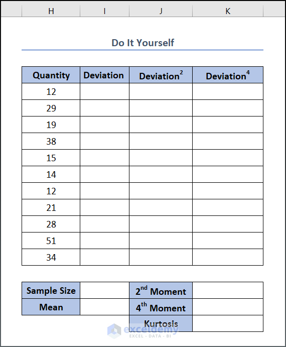
We have provided a Practice section on the right side of each sheet so you can practice yourself.
Download the Practice Workbook
You can download the dataset to practice.
Related Articles
<< Go Back to Excel for Statistics | Learn Excel
Get FREE Advanced Excel Exercises with Solutions!


How to make a graph of these values?
Hello Muhammad Azhan,
To create a graph of kurtosis values in Excel, follow these steps:
1. Create a table with your values and corresponding labels.
2. Highlight the relevant cells.
3. Go to the Insert tab >> select the desired chart type (e.g., bar or line chart).
4. Use chart tools to add titles, labels, and adjust formatting as needed.
Regards
ExcelDemy