Method 1 – Applying Trial and Error Process for Calculating Volatility in Excel
Steps:
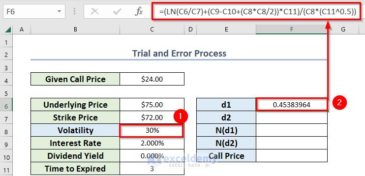
- Assume a volatility percentage in the C8. I have assumed 30%.
- In cell F6, enter the following formula to find out the d1 value.
=(LN(C6/C7)+(C9-C10+(C8*C8/2))*C11)/(C8*(C11^0.5))- Press ENTER.
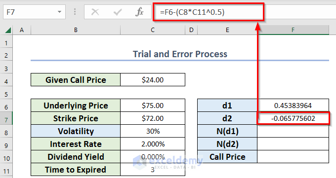
- In cell F7, enter the following formula to find out the d2 value.
=F6-(C8*C11^0.5)Press ENTER.
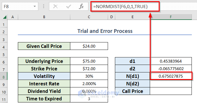
- Enter the following formula in cell F8 to find out the N(d1) value.
=NORMDIST(F6,0,1,TRUE)- Press ENTER.
Formula Breakdown:
- The NORMDIST function will return the normal distribution from the specified mean and standard deviation.
- F6 is the supplied value to calculate the distribution.
- 0 is the mean value.
- 1 is the standard deviation.
- TRUE denotes cumulative_distribution_function.
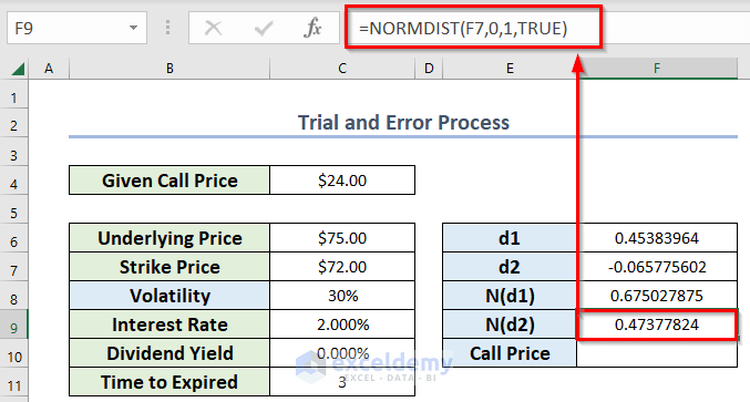
- Enter the following formula in cell F9 to find out the N(d2) value.
=NORMDIST(F7,0,1,TRUE)- Press ENTER.
- Enter the following formula in cell F10 to find out the call price.
=(C6*EXP(-C10*C11))*F8-C7*EXP(-C9*C11)*F9- Press ENTER.
Formula Breakdown:
- The EXP function will return the value of the constant e raised to the power of a given number.
- EXP(-C9*C11) gives 941764533584249.
- EXP(-C10*C11) turns 1.
- The remaining are general calculations of multiplication and subtraction.
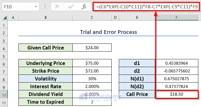
You can see that we need to compute the volatility for the call price of $24. But we have found $18 with a volatility of 30%.
Let’s find the required volatility to keep the call price at $24.
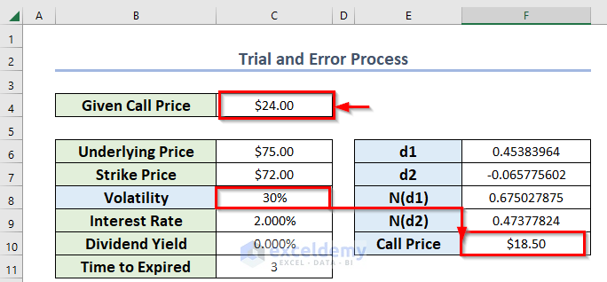
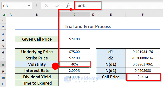
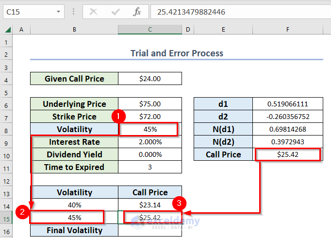
- Change the volatility percentage manually in cell C8 and notice the call price of cell F10. When you get a relevant or the nearest call price value compared to cell C4, you should consider that particular volatility percentage.
As an example, I have considered the volatility percentage of 40% as it gives the call price of $23.14 which is very close to $24.
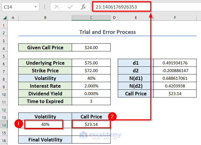
- Enter that volatility in B14.
- Enter the corresponding call price in C14.
You can use Excel keyboard shortcuts Ctrl+C and Ctrl+V to copy and paste both values.
- Choose another volatility in cell C8 to find another relevant call price.
- Enter that volatility in B15.
- Enter the corresponding call price in C15.
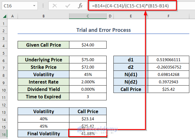
- Enter the following formula in cell C16 to find out the final volatility for the given call price.
=B14+(C4-C14)/(C15-C14)*(B15-B14)- Press ENTER to get the volatility.
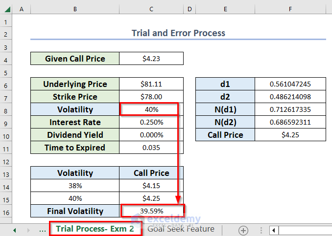
The final volatility is 39.59% for a call price of $4.23.
Method 2 – Use of Goal Seek Feature to Compute Volatility for Black Scholes
Steps:
- Assume a volatility percentage in C8 I have assumed 30%.
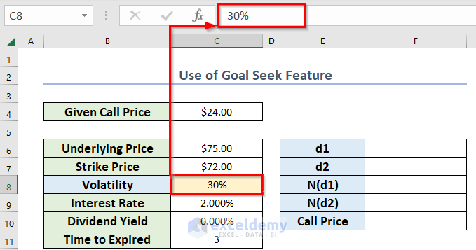
- Follow the steps in Method 1 to get the values of d1, d2, N(d1), N(d2) and call price.
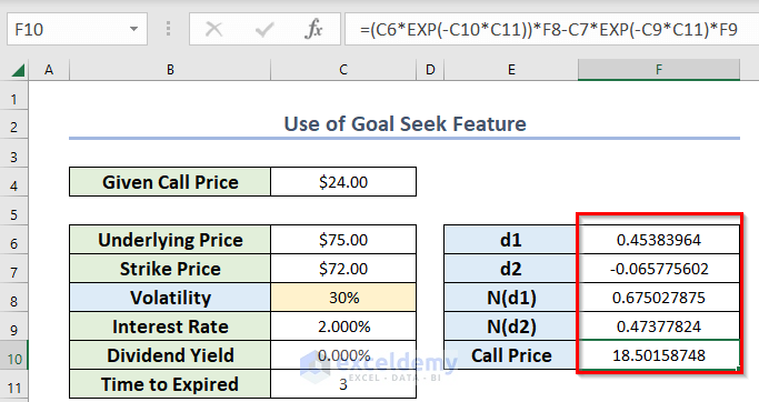
- Select cell F10.
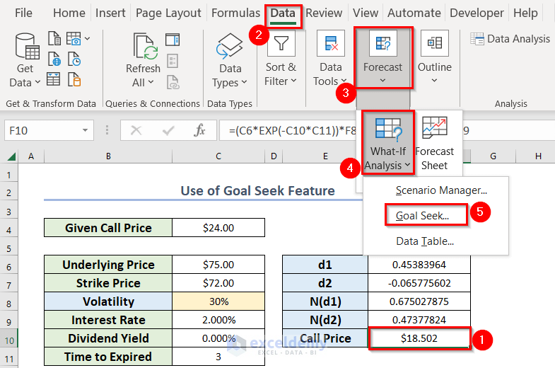
- From the Data tab >> go to Forecast >> from What-If Analysis >> choose Goal Seek.
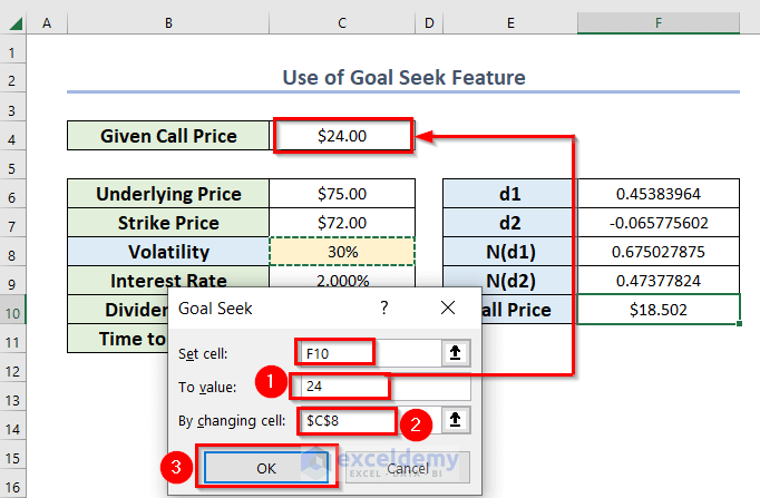
A new dialog box named Goal Seek will open.
- Select cell F10 in the Set cell box.
- Enter 24 in the To value You must enter the value which is the given call price.
- Select cell C8 in the By changing cell You must select the cell where the volatility percentage was situated.
- Press OK.
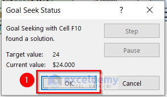
A dialog box named Goal Seek Status will pop up.
- Press OK.
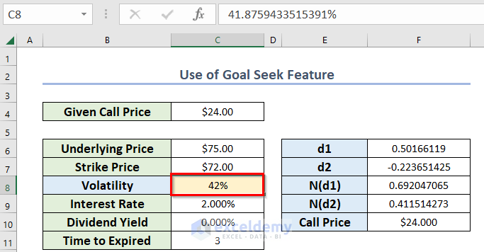
You will see the correct volatility percentage in cell C8 for the call price of $24.
Read More: How to Calculate Implied Volatility in Excel
Download Practice Workbook
Related Articles
- How to Calculate Annualized Volatility in Excel
- How to Generate Volatility Surface in Excel
- How to Calculate Historical Volatility in Excel
- How to Calculate Realized Volatility in Excel
<< Go Back to Volatility In Excel | Excel for Finance | Learn Excel
Get FREE Advanced Excel Exercises with Solutions!

