How to Convert GBP to USD in Excel (4 Suitable Methods)

When it came to the case of calculating, Excel shines with its outstanding features. Excel provides us with extraordinary features and formulas to convert the currencies according to your preference. The U.K Pound Sterling, also known as GBP, is a currency in the United Kingdom. But in this modern world, almost all accounting problems are based on the United States Dollar (USD) currency system. So, we may need to convert GBP to USD for our calculation. No need to get worried. We can perform this operation with the help of Excel’s formulas and features. In this article, we’ll show you some easy and useful methods of how to convert GBP to USD in Excel. Let’s get started.

How to Convert GBP to USD in Excel: 4 Suitable Methods

We will describe 4 very useful and effective methods to convert GBP to USD in Excel. All the methods are very easy and time-saving also. Here, we have taken a dataset of the Price of Fruit Items in GBP. We want to convert them to USD.

Here, we have used Microsoft 365 version. You can use any other version at your convenience.

1. Using Simple Arithmetic Formula

If you know the conversion rate among your converted currencies, then you can apply general arithmetic multiplication to convert the GBP to USD. You can get the conversion rate from Google. After entering the conversion rate, multiply the value with your data. Please see the below steps for better visualization.

📌 Steps:

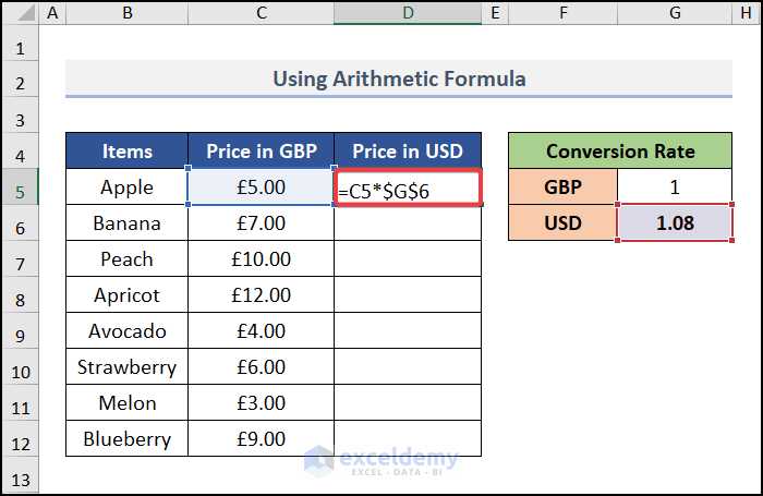
• First of all, select cell D5 and write up the formula.

Here,

C5= The cell where the prices are in GBP.

$G$6= The conversion rate of USD.

The products of this multiplication will be the converted value from GBP to USD.

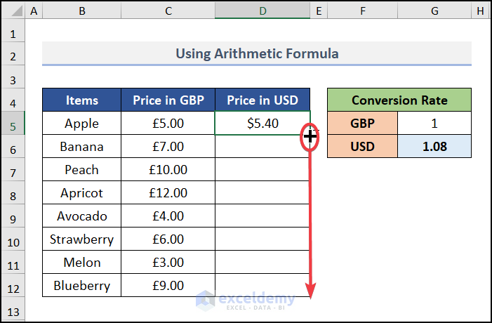
• Press ENTER and drag down the Fill Handle tool for the other cells.

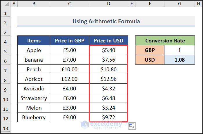
• Finally, you will get your converted result from GBP to USD.

2. Utilizing Currencies Data Type Feature

The Data Type feature is a built-in feature in Excel with which you can convert your currencies. It is a dynamic feature under the Data tab. It refreshes automatically when the price conversion rate is changed. So you can easily convert GBP to USD. We will demonstrate to you the steps for your better understanding.

📌 Steps:

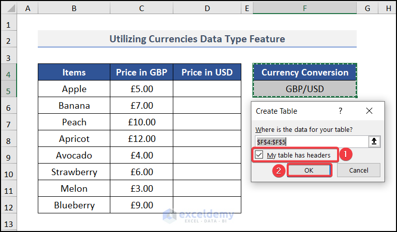
• In the very beginning, select the cells F4 and F5 to create a table for the conversion of currencies.
• After selecting the cells, go to the Insert tab >> select Table.

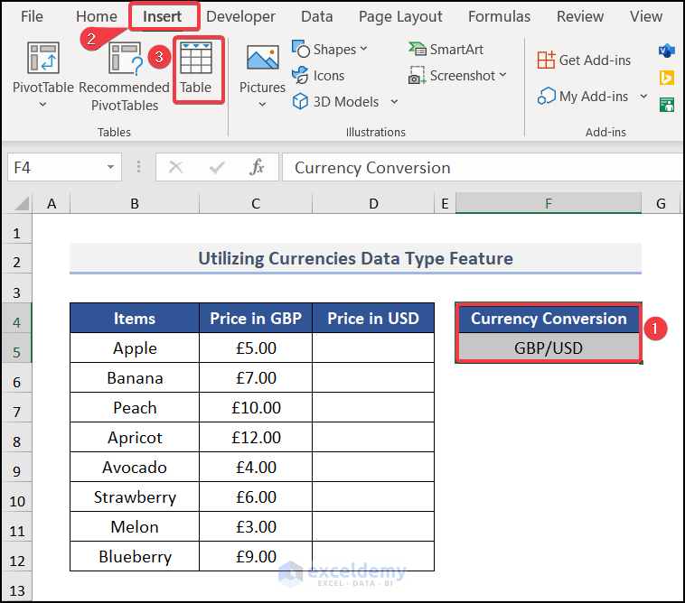
Note: You can create the table by pressing CTRL + T.

• A dialog box named Create Table will appear. Automatically, the reference cell of $F$4:$F$5 will be selected.
• Then, check the My table has headers box and press OK.

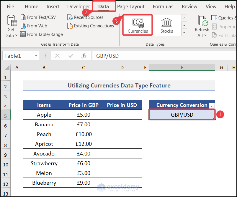
• Subsequently, move to cell F5 and select Data tab >> go to Currencies under the Data Types feature.

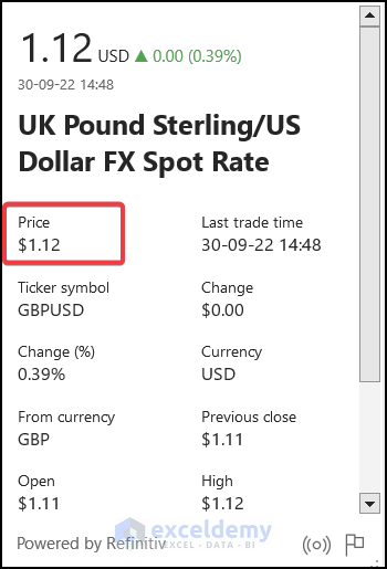
• Afterward, press CTRL + SHIFT + F5 key to open the window of UK Pound Sterling/US Dollar FX Spot Rate. Click on the Price. It will add a new column to the table.

• Consequently, go to cell D5 and write down the formula.

Here, the value in C5 will be multiplied by Table1[@Price]. Where the converted price of GBP to USD is added.

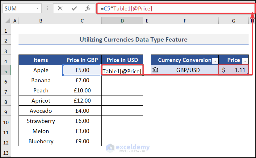
• Press ENTER and drag down the Autofill tool for other cells.

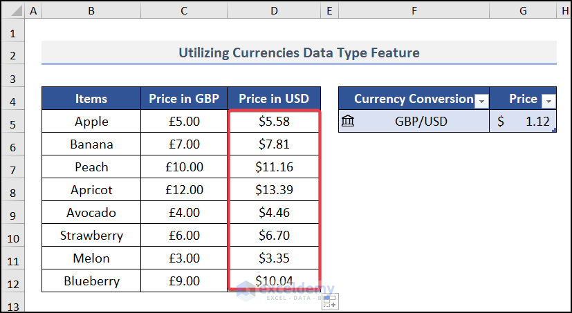
Eventually, you will be able to convert all the prices to USD.

3. Applying Power Query Feature

You can convert the currency with the help of an external data source. After inputting the XML  data available online, we will use the Power Query feature. The Power Query Editor will show you the path to load the currency conversion data in our worksheet. Follow the steps to convert GBP to USD with the help of the Power Query feature.

📌 Steps:

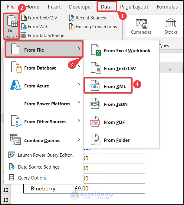
• Firstly, go to the Data tab >> select Get Data >> click on From File >> move to From XML.

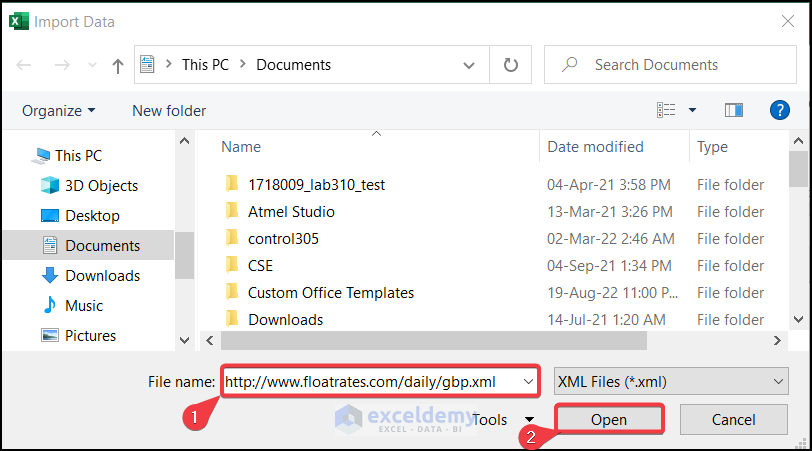
• An Import Data window will appear. Then enter the suitable URL of an XML file and hit Open.

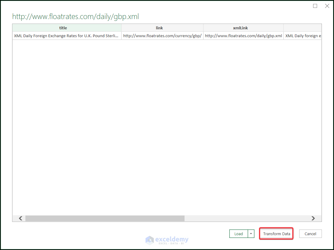
• The following window will pop out like the image and then select Transform Data.

• Gradually, gbp-Power Query Editor will open.
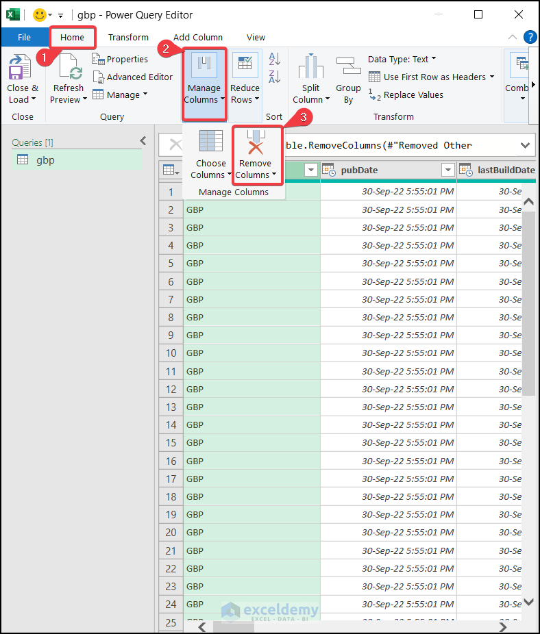
• Subsequently, go to the Home tab >> click on Manage Columns >> select Remove Columns to remove the columns you don’t need.

• After that, go to Close & Load and select it.

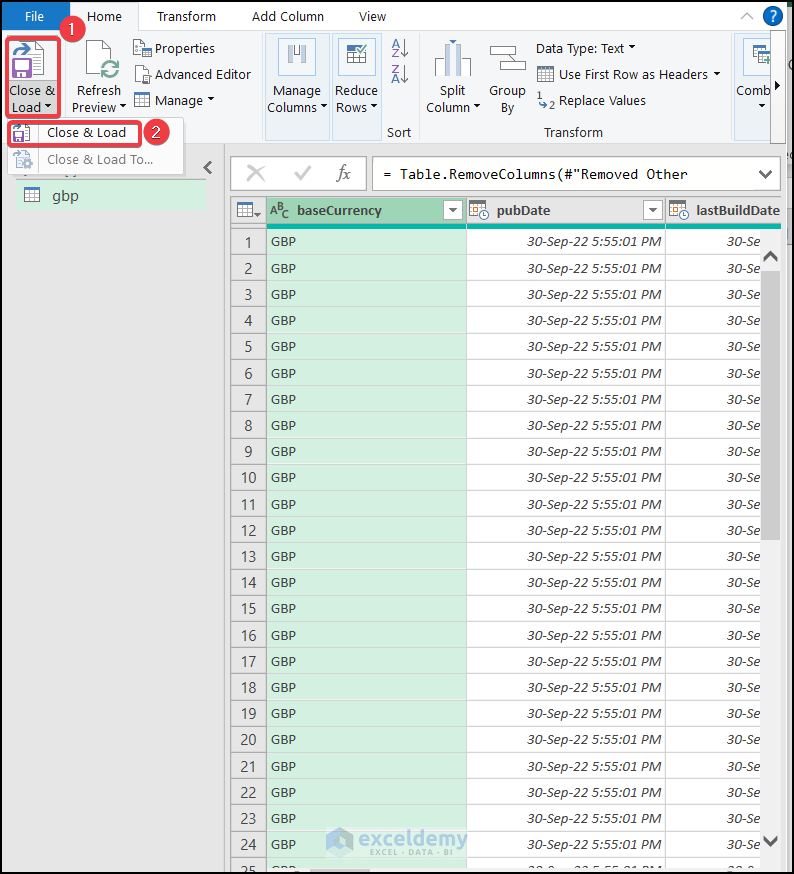
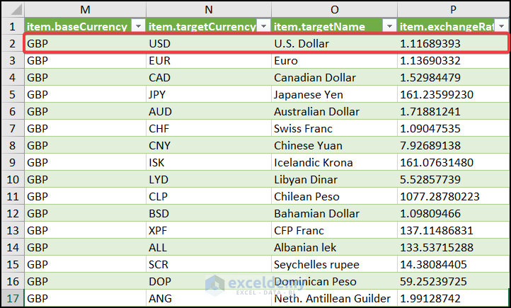
• Gradually, a new worksheet will be created named gbp and you can see all the exchange rates loaded on the sheet.

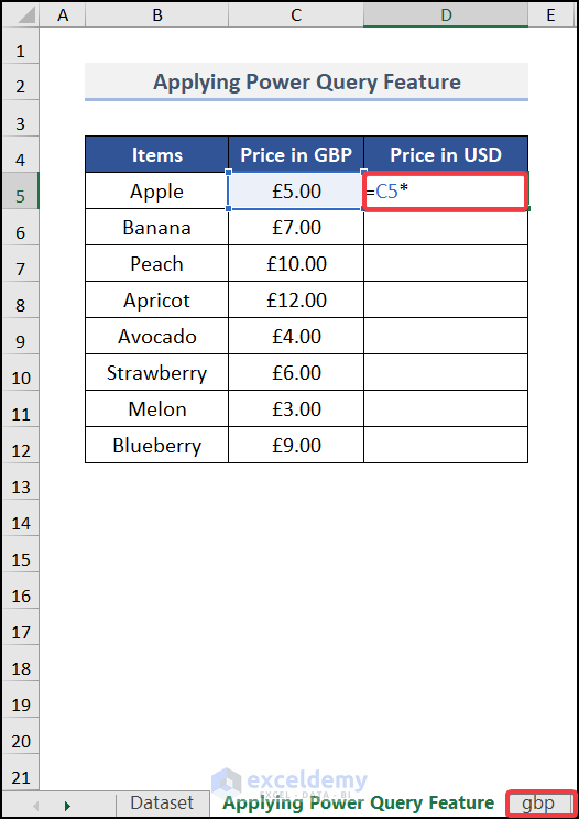
• Now, select cell D5 and enter cell C5 and a multiply sign (*) and select the worksheet gbp.

• After that, select cell P2 where the conversion rate from GBP to USD has existed.

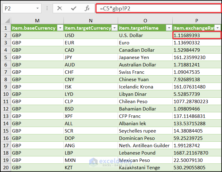
• Finally, the formula will be

• Press ENTER key and drag it down for other cells.

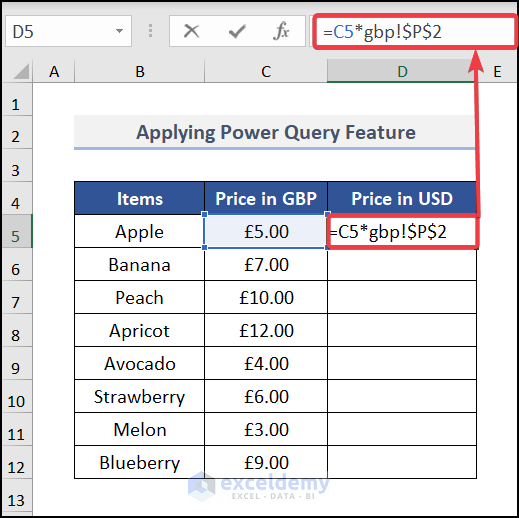
Note: Don’t forget to lock the cell reference by pressing F4 key.

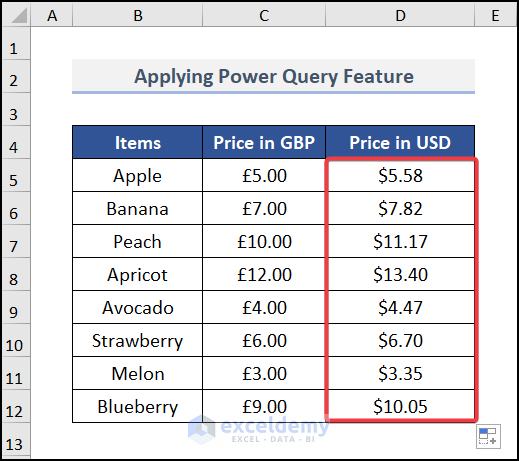
• Finally, you will get your desired result.

4. Utilizing VLOOKUP Formula

We can also use the Excel formula to convert the currency from GBP to USD. All we need to enter is the conversion rate that is acquired from Google. Then we will apply the VLOOKUP function for the conversion. Follow the simple steps we have discussed below.

📌 Steps:

• Firstly, select cell D5 and insert the formula stated below.

Here,

$F$5= The lookup cell where we enter the text USD.

$F$8:$G$9= The entire range of Conversion Rate.

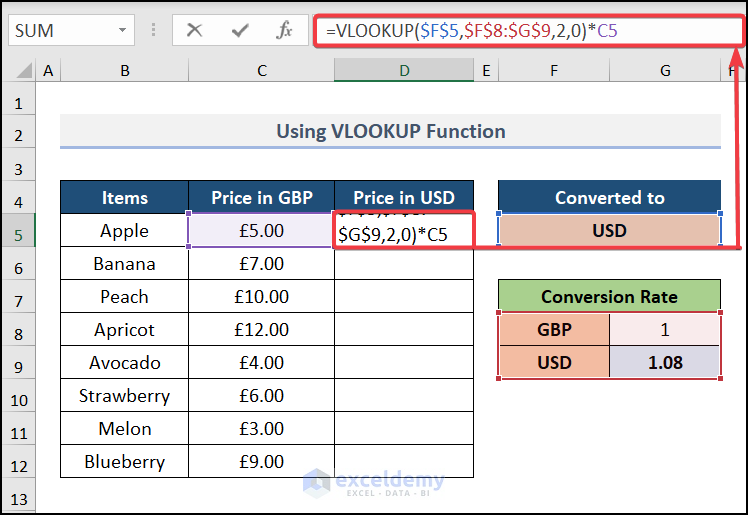
• Press ENTER and drag down for the same formula in other cells.

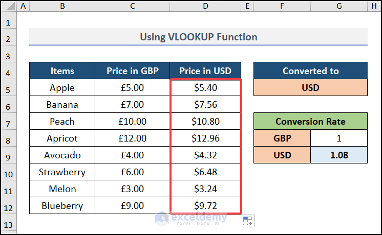
• Lastly, you will get the result.

Similarly, you can also apply the Nested IF and INDEX & MATCH functions for converting GBP to USD in Excel.

Practice Section

We have provided a practice section on each sheet on the right side for your practice. Please do it by yourself.

Download Practice Workbook

Download the following practice workbook. It will help you to realize the topic more clearly.

Conclusion

That’s all about today’s session. And these are some easy methods on how to convert GBP to USD in Excel. Please let us know in the comments section if you have any questions or suggestions. For a better understanding please download the practice sheet. Thanks for your patience in reading this article.

<< Go Back to Currency Conversion in Excel | Learn Excel