How to Copy and Paste Without Changing the Format in Excel: 4 Methods

Method 1 – Quickest Method: Use the ‘Keep Source Column Widths (W)’ Command

Step 1: Select source cells B6:C16 and press Ctrl+C to copy them.

3 Ways to Copy Cells in Excel

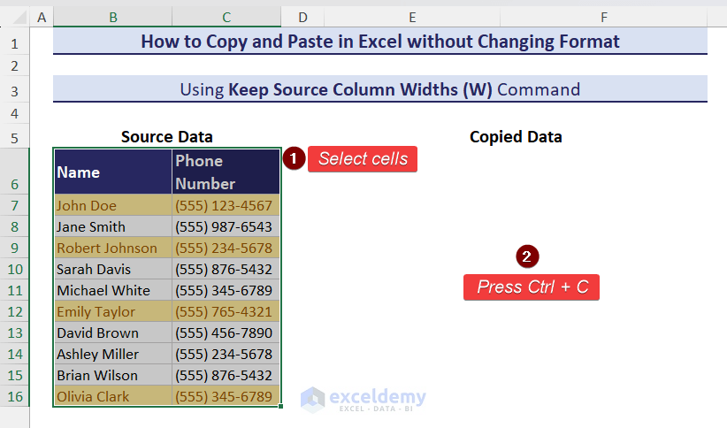
Select cells ⇒ press Ctrl+C.
Select cells ⇒ Clipboard group of commands ⇒ Click the Copy button.
Select cells ⇒ Right-click your mouse ⇒ Click Copy.

Step 2: Click on cell E6 ⇒ Clipboard ⇒ Paste drop-down.

Step 3: Choose the Keep Source Column Widths (W) option from the appeared options.

Note:
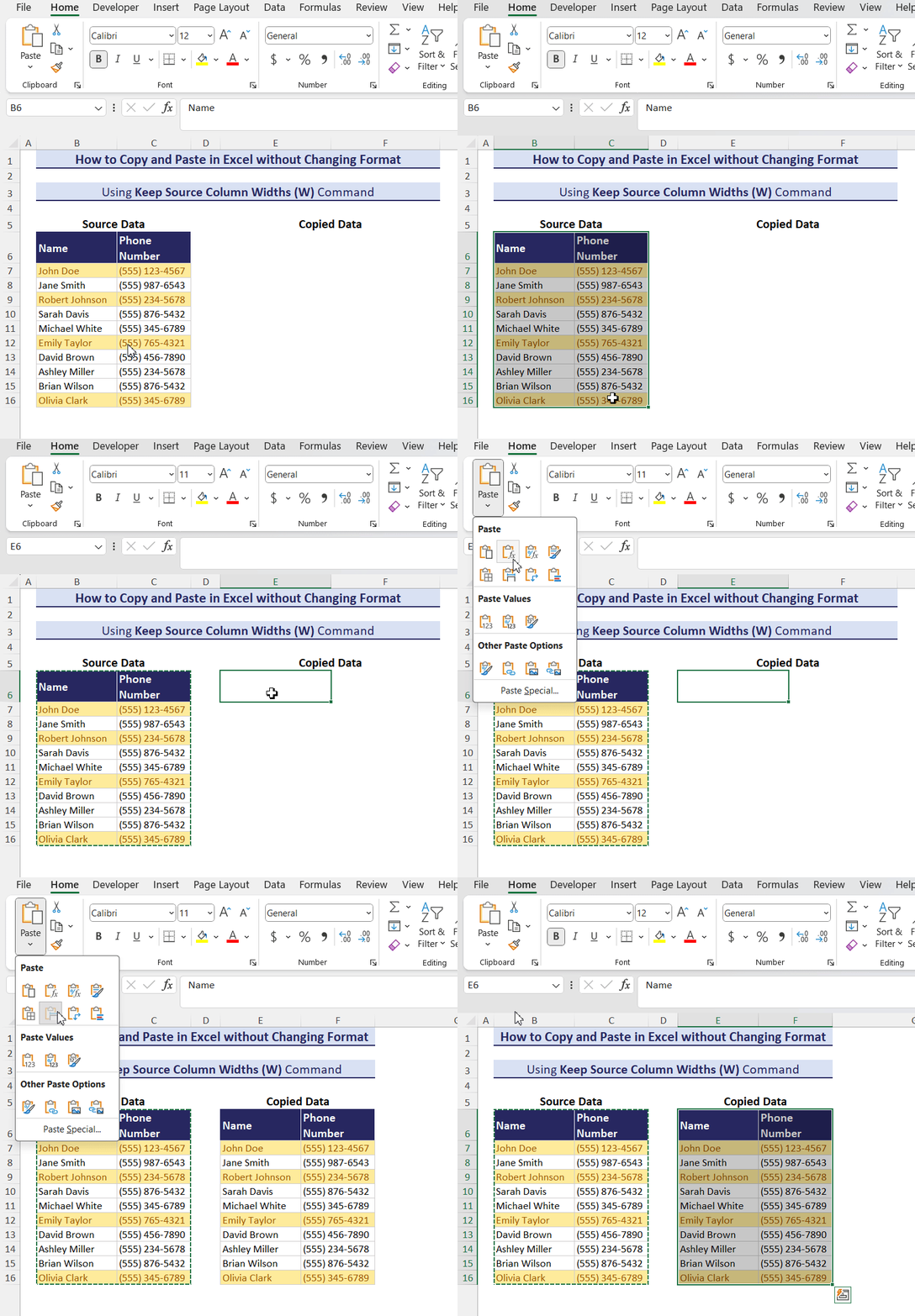
To copy and paste without changing the format, use the Keep Source Column Widths (W) command from the context menu.

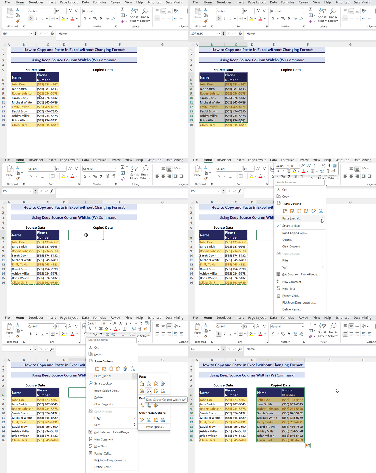
Method 2 – Adjust Column Widths Using Paste Options Button after Pasting Cells, Keeping Source Cells’ Format Intact

To copy and paste without changing the format, use the Paste command from the Clipboard group of commands and context menu. Apply a keyboard shortcut. After copying cells, the column widths are not usually copied, so you may not see data sometimes.

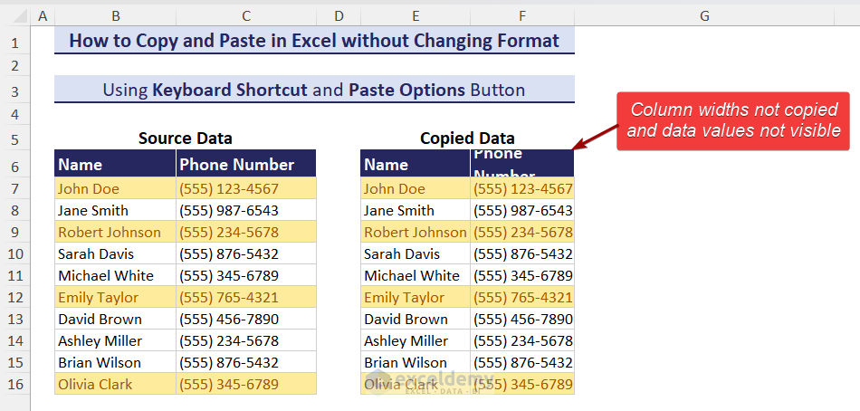
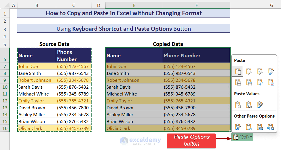
Once you have pasted cells, you can use the Excel Paste Options button, which appears when you copy and paste. It is in the bottom right corner of the destination cells.

How to Enable Paste Options Button?

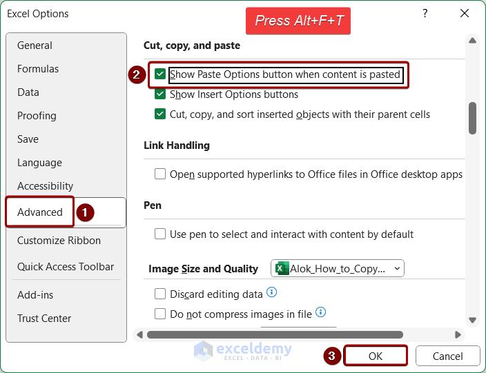
Go to File ⇒ Options or press Alt + F + T ⇒ Advanced option ⇒ Cut, copy, and paste section ⇒ Check the Show Paste Options button when content is pasted option.
Press the OK button.

See the whole method step by step.

Step 1: Select range B6:C16 and press Ctrl+C to copy the cells.

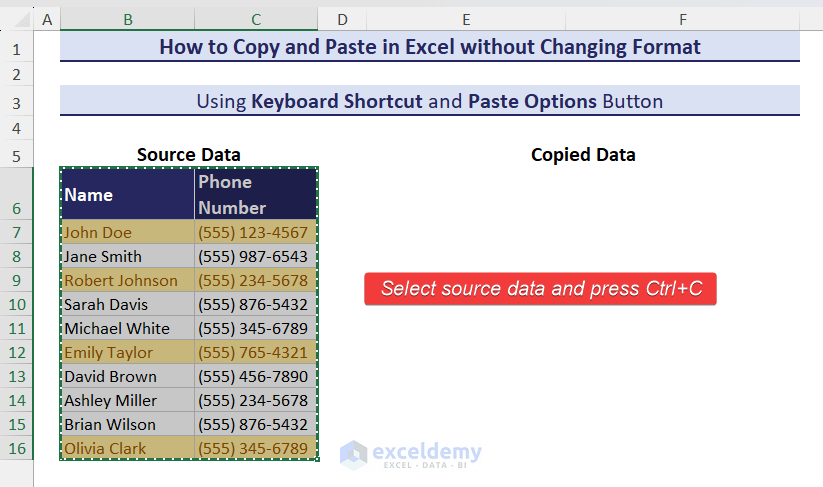
The dotted line around the selected range indicates that our data has been copied to the clipboard.

Step 2: Move the cursor to the destination range’s first cell, cell E6.

Step 3: Press Ctrl+V.

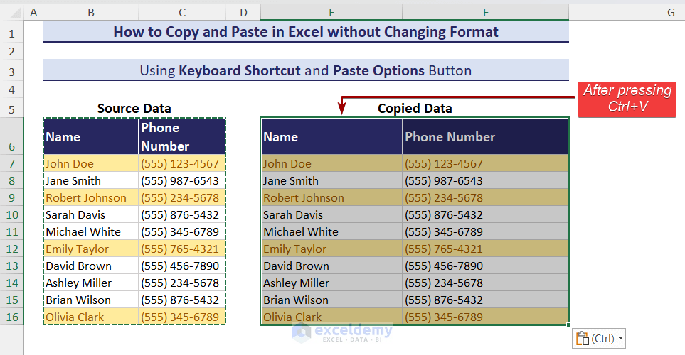
Step 4: Click on the down arrow of the Ctrl button at the right-bottom side on the pasted data. Click the Ctrl button from the keyboard.

Step 5: From the Paste Options dialog box, click the Keep Source Column Widths (W) option.

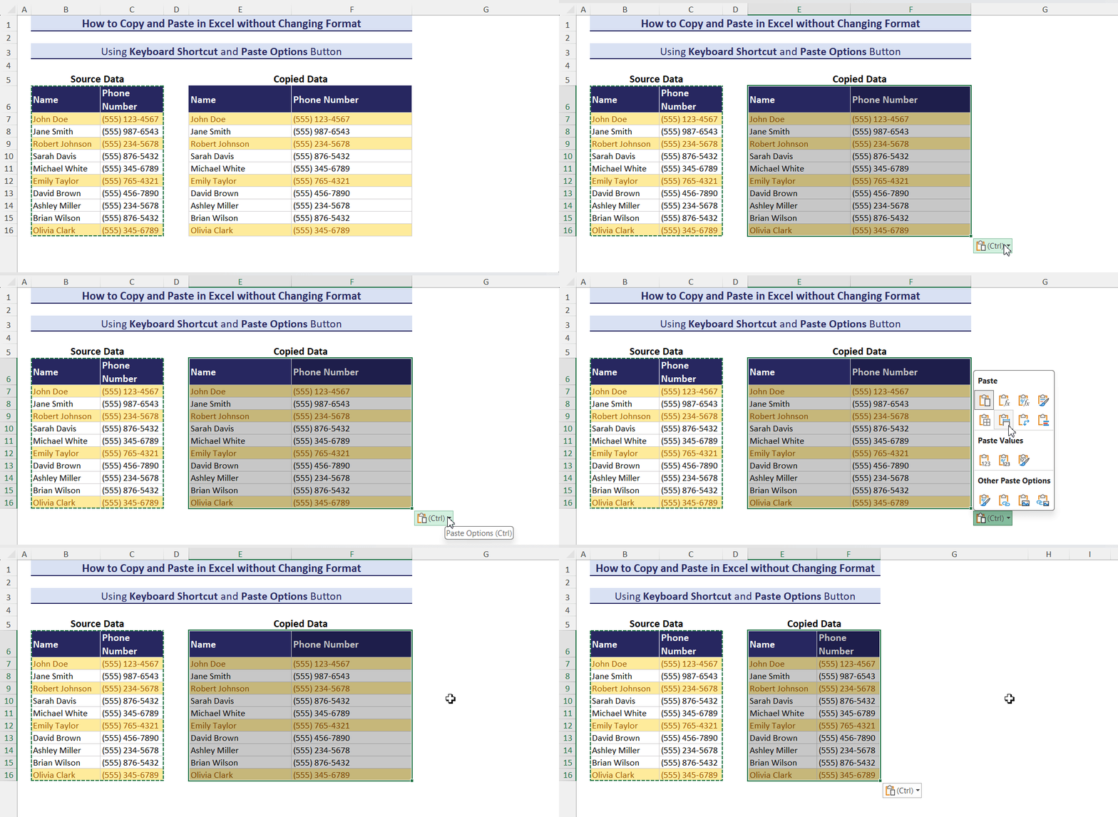
The column width of the pasted data is the same as the source data. In the below section, we will show more ways to copy and paste the Paste Options button in Excel without changing the format.

2 More Ways to Paste Cells in Excel

You can also paste cells keeping the previous cells’ formatting in the following 2 ways. Use the Keep Source Column Widths (W) option from the Paste Options button to make the column width the same as the source cells.

Copy B6:C16 ⇒ Move to cell E6 ⇒ go to Home ⇒ Clipboard group ⇒ Click Paste.

Or,

Copy range B6:C16 ⇒ Move to cell E6 ⇒ right-click your mouse ⇒ Choose Paste (P) from the Paste Options section of the context menu.

Method 3 – Using Paste Special Dialog Box to Copy and Paste Keeping Format Unchanged

Step 1: Copy the source data.

Step 2: Move to cell E6 and click the down arrow of the Paste option from the Clipboard group.

Step 3: Click the Paste Special option from the shown options.

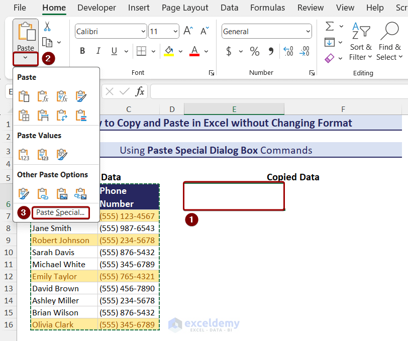
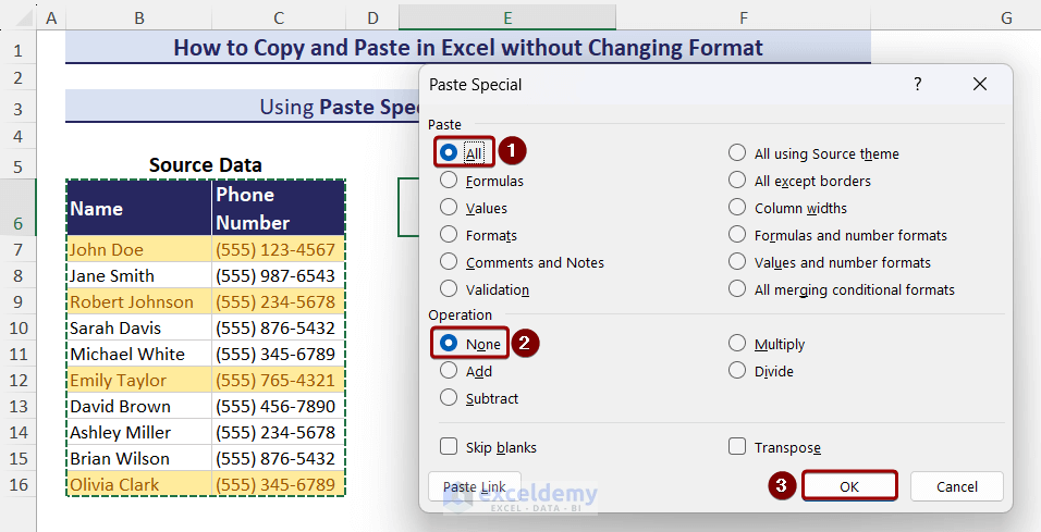
The Paste Special window appears.

Step 4: Select All in Paste and None in the Operation section (the default options).

Step 5: Click the OK button.

Data has been pasted, but cell width is not the same.

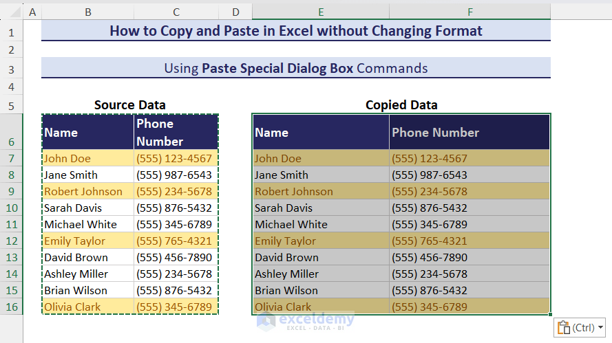
Use the Paste Special option to keep the cell width intact.

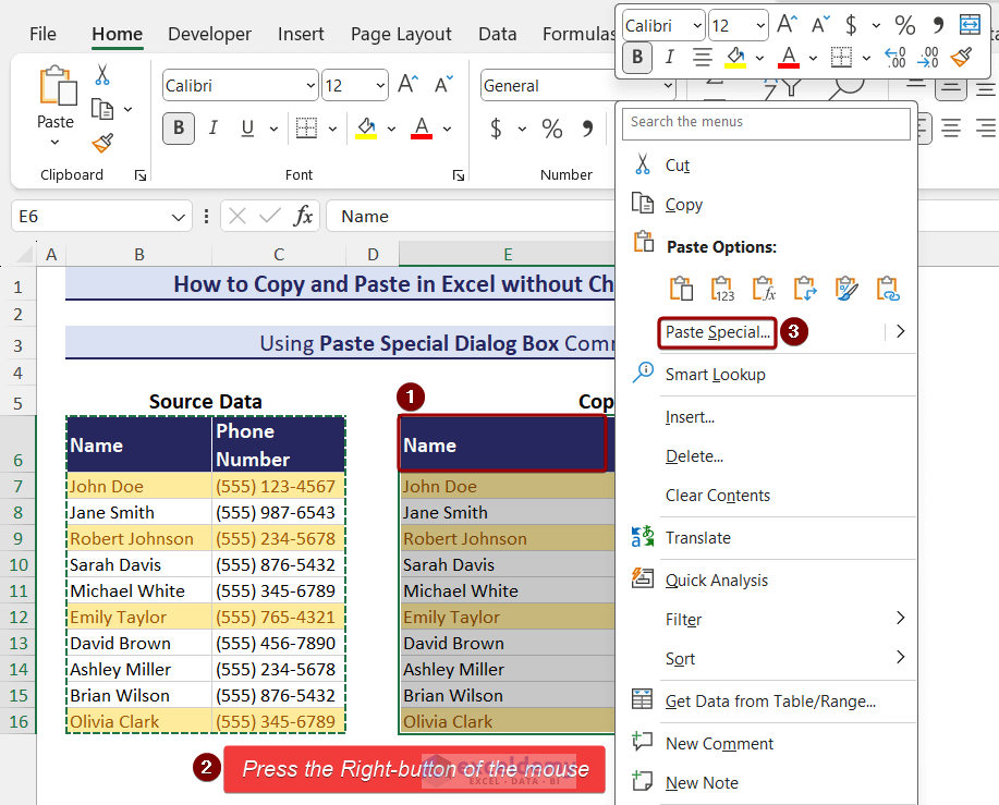
Step 6: Move to the first cell of the pasted data, cell E6, and press the right button of the mouse.

Step 7: Choose the Paste Special option from the Context Menu.

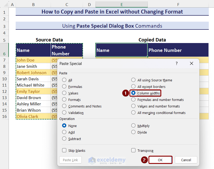
Step 8: Choose the Column widths option in the Paste section and click the OK button.

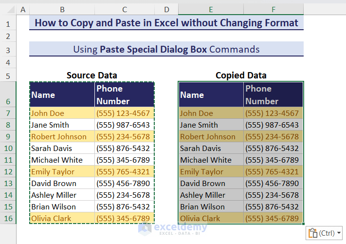
See the cell width of the pasted data; it is the same as the source data.

Method 4 – Mouse Tricks to Copy and Paste in Excel Without Changing the Format (Except for Column Width)

i. Dragging with the Right Mouse Button

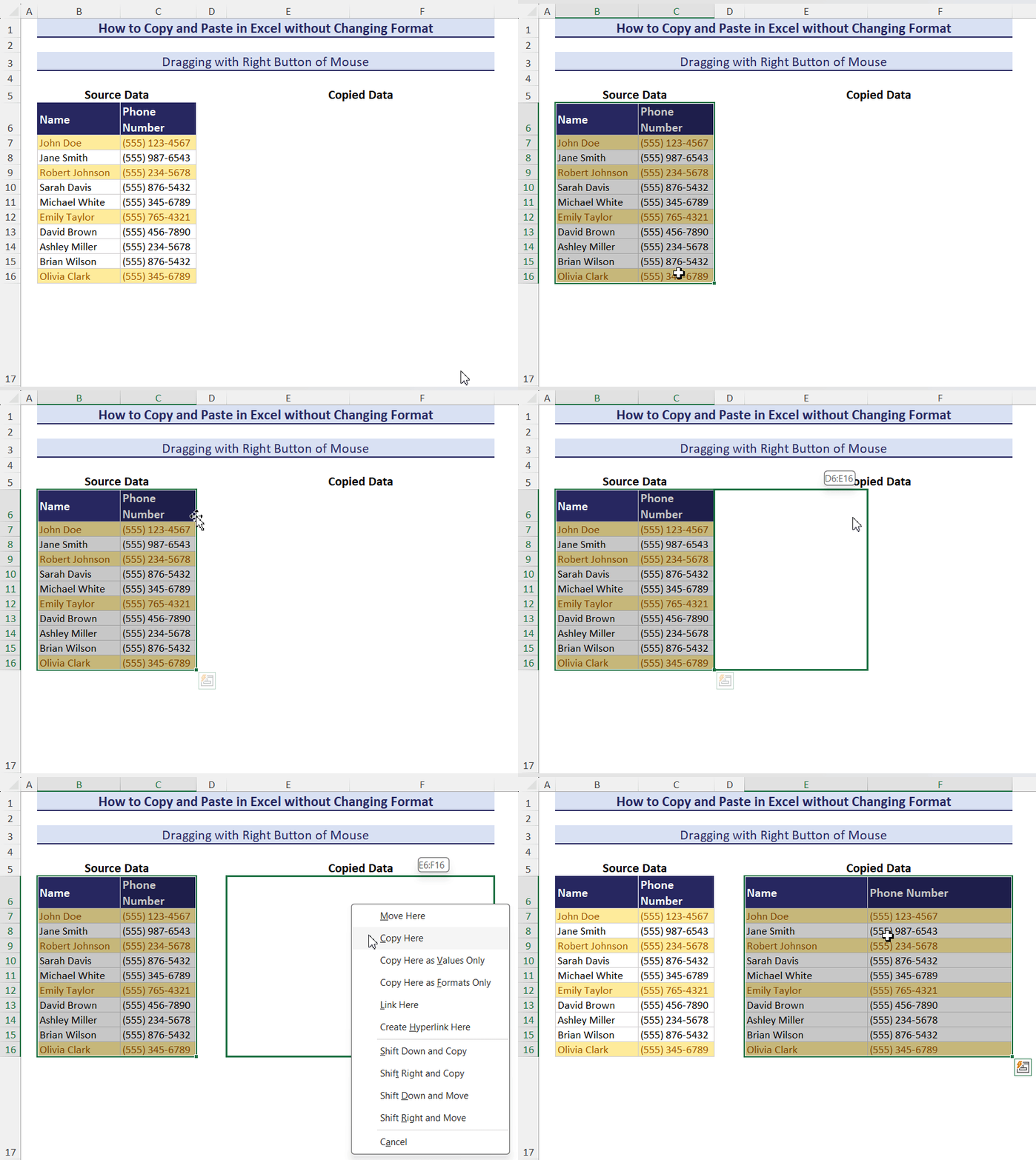
Select range B6:C16.
Move the mouse to the edge of the selection range and wait until the four-directional sign appears.
Click and hold the right button of the mouse and drag the mouse to a space to paste.
Release the mouse button, and a menu will appear.
Click the Copy Here option, and data will be pasted from the source.

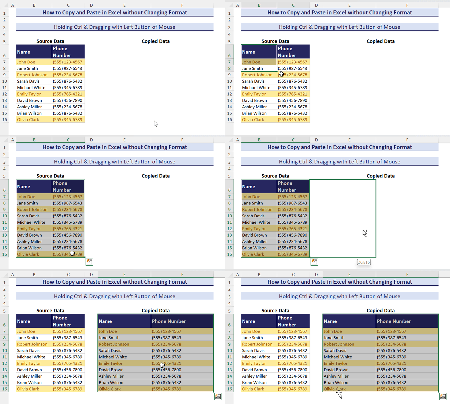
ii. Press and Hold the Ctrl Key and Drag with the Left Mouse Button

Select range B6: C16 and hold the Ctrl key.
Move the cursor to any edge of the dataset and wait until the small plus (+) symbol appears.
Click the mouse’s left button and drag the cursor to an empty cell.
Release the left button to see the data being pasted to the new location.

Download Practice Workbook

Copy and Paste Without Changing the Format.xlsx

<< Go Back to Copy Paste in Excel | Learn Excel

Get FREE Advanced Excel Exercises with Solutions!

2 Comments

Paresh Kanti Paul Dec 10, 2024 at 4:58 PM

Date: 10 December, 2024.
Dear Sir,
Ref. http://www.ablebits.com/excel-suite/trim-spaces.php

How do I copy-paste such kind of screenshot captured Excel Data Table in Excel Worksheet (as shown in above website–Staff List)?
Looking forward to get an answer.
Best regards,
Paresh Kanti Paul
Chittagong.
- Reply
  Shamima Sultana Dec 11, 2024 at 11:53 AM
  
  Hello Paresh Kanti Paul,
  
  Thank you for reaching out. To copy and paste a screenshot of an Excel Data Table (like the one shown on the mentioned website) into an Excel worksheet, you can follow these steps:
  
  Take a Screenshot: Use the Snipping Tool (Windows) or Command + Shift + 4 (Mac) to capture the table as an image.
  Paste into Excel: Open your Excel worksheet, right-click where you want to insert the image, and choose Paste (or press Ctrl + V).
  Adjust Image: You can resize or move the image as needed within the worksheet.
  
  If you’d like to recreate the data as an editable table (instead of a static image), you can try these options:
  
  If you want to convert an image of a table into an editable Excel table, Excel Desktop also has a Data from Picture feature (previously available only on mobile).
  Here’s how you can do it:
  1. Go to the Data tab in Excel Desktop.
  2. Click From Picture and select Picture From File or Picture From Clipboard.
  3. Excel will process the image and convert it into an editable table.
  
  Regards
  ExcelDemy