How to Display Exponents in Excel: 7 Simple Methods

Method 1 – Using Superscript Effect

To display exponents by applying the Superscript effect, follow the steps:

1. Insert the values of Number and Power together in a new range.
   If the number is 2 and the power is 3, it would be 23.
   
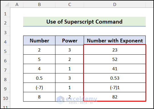
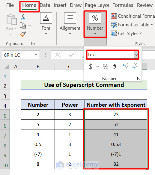
2. Select the new range.
3. Go to the Home tab > Number group > Number Format dropdown > Text.
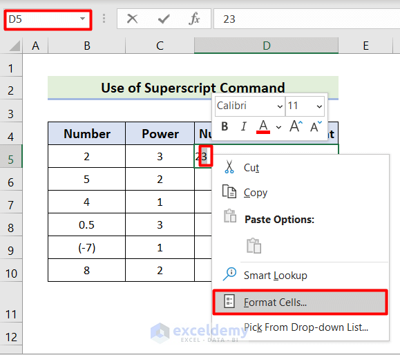
4. Double-click on the first cell and select only the Power characters.
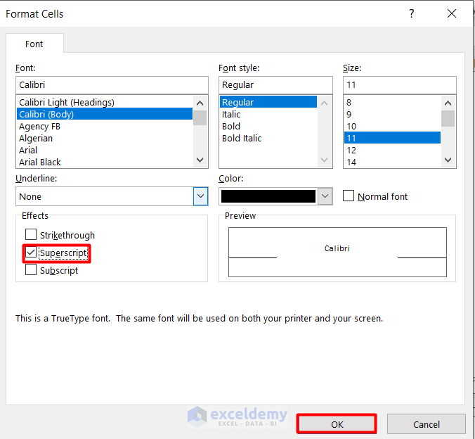
5. Right-click and select Format Cells.The Format Cells dialog box will appear.
6. Go to Font tab > Superscript effect > OK.
7. Press Enter, and the exponent will be displayed in the first cell.
   
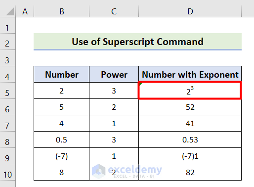
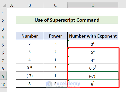
8. Similarly, implement the same procedure in other cells to get the final output.

Method 2 – Using Superscript Button from Quick Access Toolbar

To add the superscript button and use it to display exponents, follow these steps:

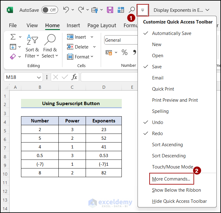
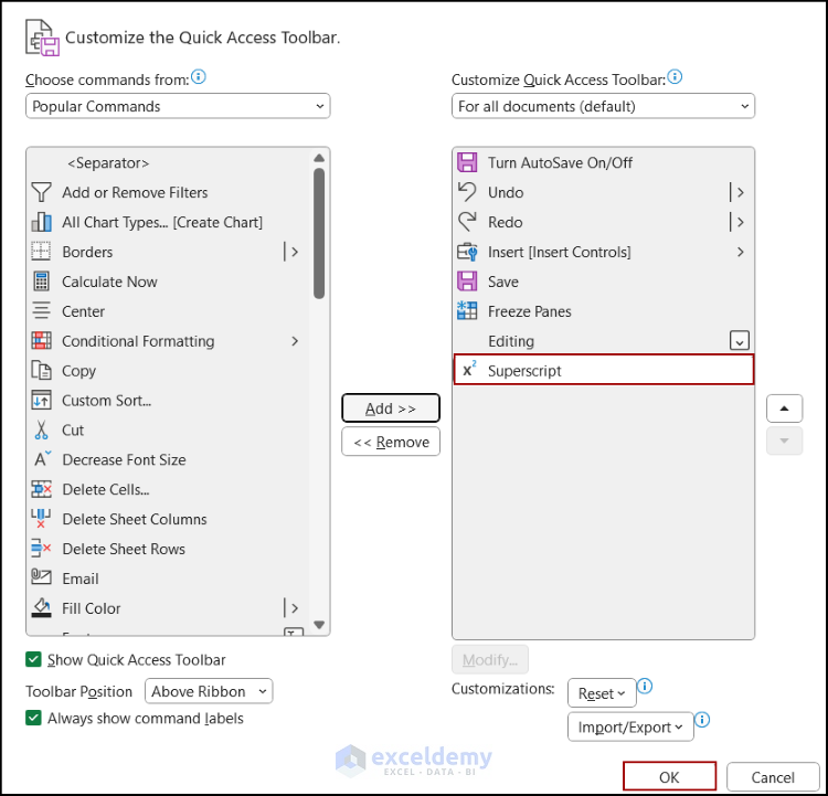
1. Click on the Customize Quick Access Toolbar dropdown > More Commands.
   A dialog box named Customize the Quick Access Toolbar will pop up.
2. Under Choose commands from option > Commands Not in the Ribbon > Superscript command > Add.
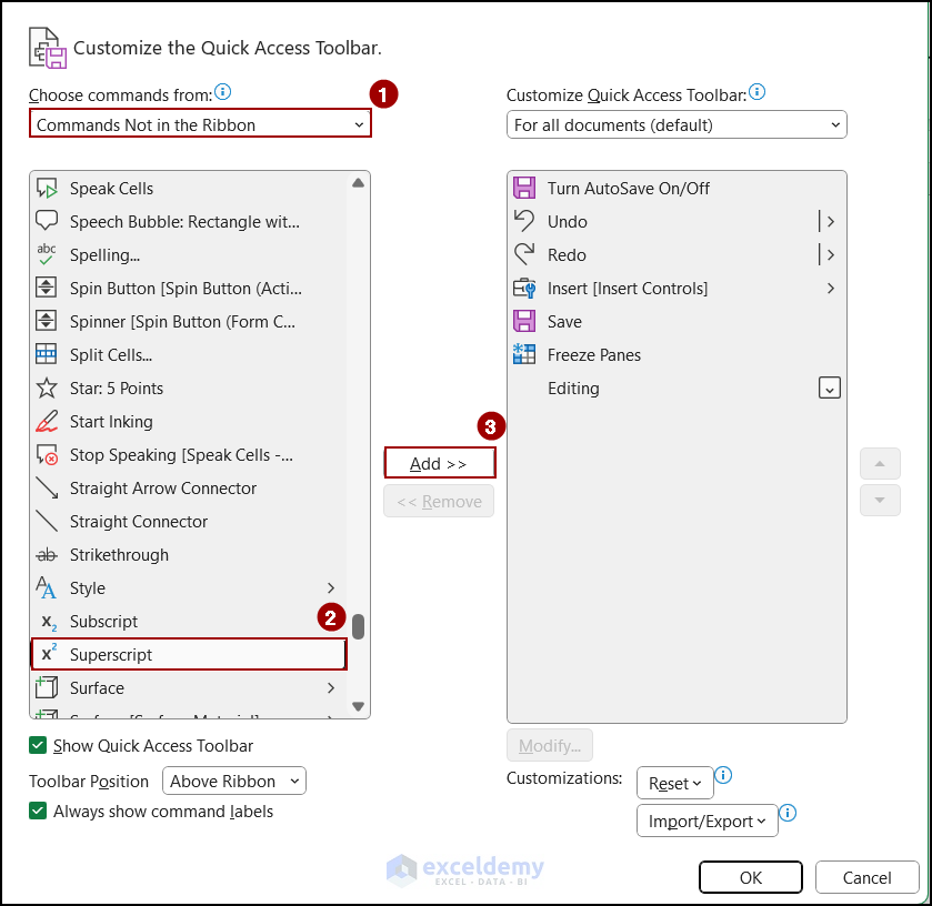   The Superscript command will be shown on the right side.
3. Press OK.
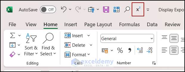
   You can see the superscript icon on the Quick Access Toolbar.
   
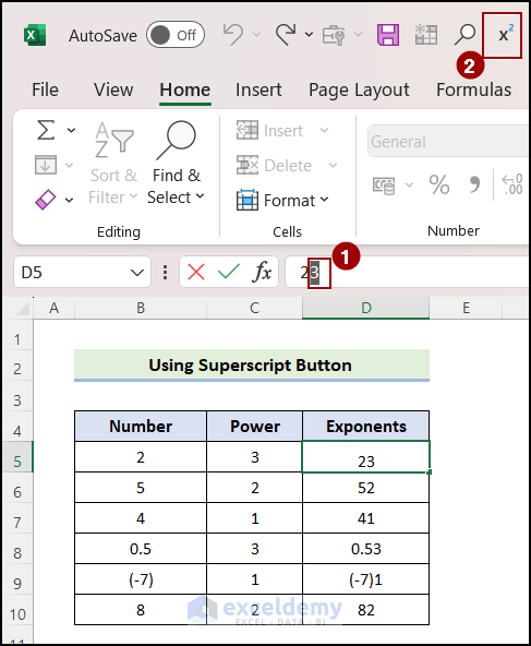
4. Select the power character and click on the Superscript button from the Quick Access Toolbar.
   The selected cell should be in Text format.
   
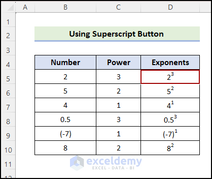
5. The exponent will be displayed. Follow the same process for the rest of the cells.
   

Method 3 – Using Custom Format

The Custom format in Excel alters only the visual representation of numbers inside a cell. The value contained in a cell’s underlying location is not changed. It is not possible to alter or erase the original number format.

To use a custom format to show exponents, follow the steps below:

1. Copy the Number range and paste it into a new range.
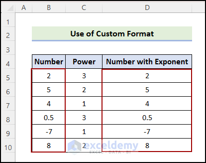
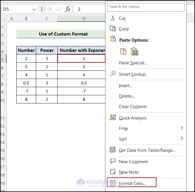
2. Select first cell in the new range and right-click.
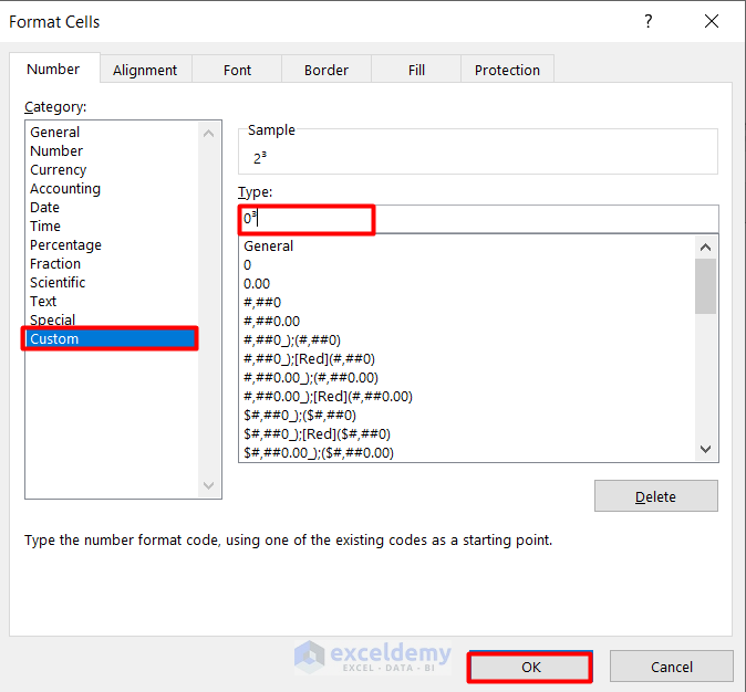
3. Select Format Cells.The Format Cells dialog box appears.
4. In the Format Cells dialog box:
   • Go to Category > Custom.
   • Type 0 in the Type box.
   • Hold the Alt key and type 0179 for exponent 3, or 0178 for exponent 2, or 0185 for exponent 1.
   • You have to use numerical keys for this, the number insertion may not work.
   • Click OK.

   

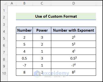
5. Repeat the same procedure for other cells to get the final result:

Method 4 – Using Insert Equation Feature

The Insert Equation feature provides an advanced solution for crafting professional and well-formatted equations in Excel. It cannot be directly applied to a cell; instead, you can create the equation in a text box and manually place it within it.

The steps required for displaying exponents using the Insert Equation feature are given below:

1. Go to the Insert tab > Symbols > Equation.
2. Go to Script > Subscripts and Superscripts > Superscript.
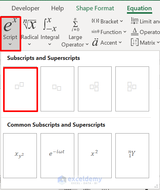   A box will appear to take inputs.
3. Next, type the base Number and the Power.
   In this case, 2 and 3, respectively.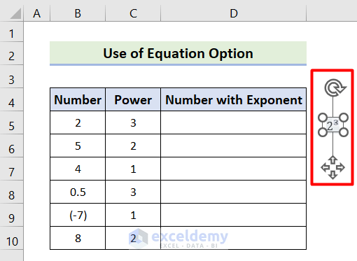
4. Move the box to a cell.
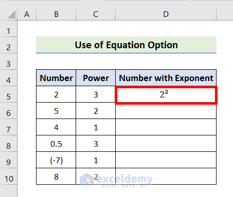
5. Use the same procedure for other cells.

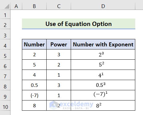
Method 5 – Using Keyboard Shortcut

Using Keyboard shortcuts allows you to show exponents without using any formulas. You can use exponents of 1, 2, and 3 using this method. You must hold the Alt key down for this.

Follow the instructions below to display exponents using a keyboard shortcut:

1. Double-click a cell containing a number to enter edit mode.
2. Hold the Alt key and using numerical keys, press any of the following keys:
   • To insert the exponent of 3 press 0179.
   • For inserting the exponent of 2 press 0178.
   • To insert the exponent of 1 press 0185.

   

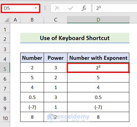
3. Do the same for other numbers.

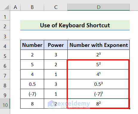
Note: If you don’t enter edit mode, the corresponding exponent will replace the cell content.

Method 6 – Applying Excel Functions

The CHAR and UNICHAR functions can display exponents in Excel. These functions use ASCII and Unicode, respectively, to return characters.

Here are 2 methods to display exponents using Excel functions:

Method 1: Using CHAR Function

The CHAR function returns a character based on its ASCII code. Exponents are superscripts and are not available to input from the keyboard. In such cases, you can display the exponents based on the number you provided as ASCII code for the CHAR function argument.

To display exponents by applying the CHAR function, follow the steps:

1. Select a cell.
2. Insert the following formula: =B5&CHAR(179)
   Use ASCII codes 185, 178, and 179 for exponents 1, 2, and 3, respectively.
3. Click on Enter.
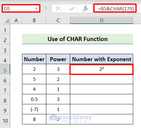
4. Follow the same procedure for other cells.

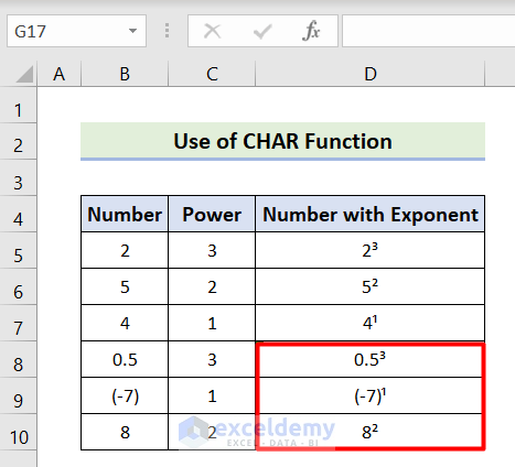
Method 2: Applying UNICHAR Function

Although the CHAR function is quite useful, it has a noticeable limitation. The CHAR function can return characters corresponding to ASCII codes from 1 to 255. As a result, it can’t display superscripts of more than 3.

In such cases, applying the UNICHAR function can be beneficial as it uses Unicode and can display superscripts beyond basic numerals 0-9. The UNICHAR function is supported in Excel 2013 and later versions.

To apply the UNICHAR function to display exponents, follow the steps:

1. Select a cell.
2. Insert the following formula:=B5&UNICHAR(8310)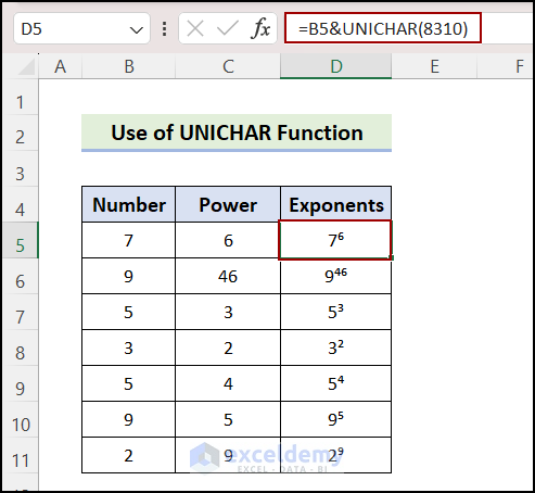This returns an exponent of 6. If the exponent contains multiple characters, you have to use multiple UNICHAR functions.
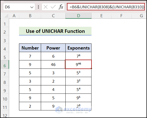
3. For example, to get the exponent of 46 insert the following formula: =B6&UNICHAR(8308)&(UNICHAR(8310))
   8308 and 8310 refer to Unicode values for exponents of 4 and 6.

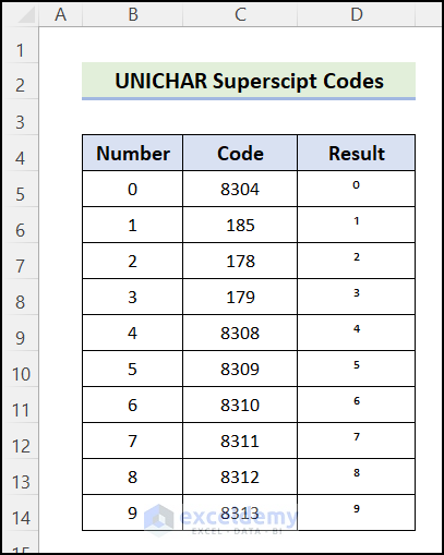
The following image displays the UNICHAR codes for corresponding superscripts:

Method 7 – Using VBA User Defined Function

Excel VBA offers a powerful and automated solution for displaying exponents. By utilizing VBA, users can create personalized scripts to effortlessly insert exponents into cells, streamlining the entire process and ensuring uniformity.

Using VBA to display exponents is particularly advantageous when working with extensive datasets, intricate calculations, or when repeated exponent formatting is required, as it saves both time and effort compared to manual interventions.

Follow the steps below to use VBA to display exponents in Excel:

1. Go to the Developer tab > Visual Basic.
   
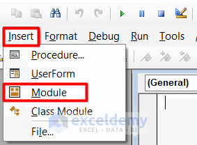
2. Go to Insert > Module.
   
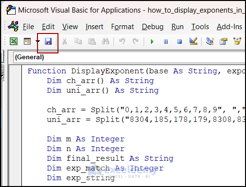
3. Insert the following code in the new module:

   Function DisplayExponent(base As String, exponent As String) As String
   Dim ch_arr() As String
   Dim uni_arr() As String
   
   ch_arr = Split("0,1,2,3,4,5,6,7,8,9", ",")
   uni_arr = Split("8304,185,178,179,8308,8309,8310,8311,8312,8313", ",")
   
   Dim m As Integer
   Dim n As Integer
   Dim final_result As String
   Dim exp_match As Integer
   Dim exp_string
   
   final_result = base
   
   For m = 1 To Len(exponent)
   exp_match = -1
   exp_string = Mid(exponent, m, 1)
   
   For n = LBound(ch_arr) To UBound(ch_arr)
   If ch_arr(n) = exp_string Then
   exp_match = n
   Exit For
   End If
   Next n
   
   If exp_match = -1 Then
   final_result = "Exponent not available"
   Exit For
   End If
   
   final_result = final_result & ChrW(uni_arr(exp_match))
   Next m
   
   DisplayExponent = final_result
   
   End Function

4. Save the code by selecting the Save icon.
5. Select the cell where you want to display the exponent.
6. Write the formula: =DisplayExponent(B5,C5)
   You’ll get the desired output.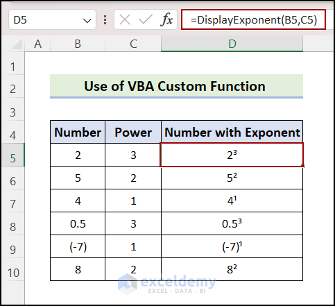

How to Display Exponents Using Scientific Notation in Excel

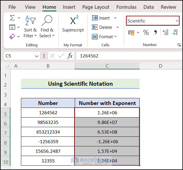
To apply the scientific format to a number in Excel:

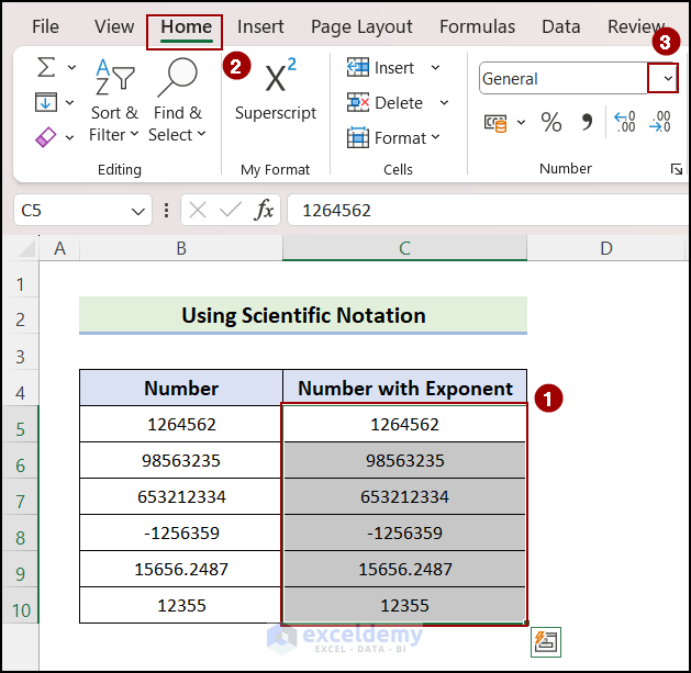
1. Select the range you want to display as an exponent.
2. Go to the Home tab > Number group > Number Format drop-down.
   
3. Choose Scientific.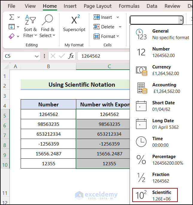All the selected numbers will be displayed as exponents now.
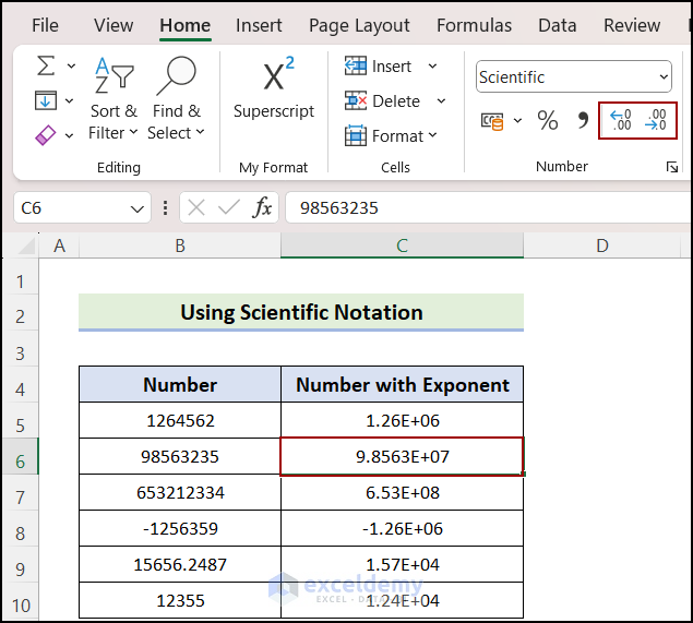
4. Use the arrows in the Number group to specify the number of decimal places you want to display.

Notes:

• Changing the Number Format does not change the actual value. You can see the actual value in the formula bar.
• Excel has a precision limit of 15 digits, so very large numbers may be displayed differently in the formula bar.
• To remove scientific notation for large numbers, set the Number Format to Number.

Download Practice Workbook

Please receive a free copy of the example workbook utilized during the session.

Frequently Asked Question

How to display exponents in Excel charts?

If you want to display exponents from source data in charts, you may get normal characters instead. This usually happens if the superscript in the dataset is inserted by enabling the Superscript effect from the Font tab of the Format Cells dialog box.

You can insert superscripts in the source data from the Symbol feature to get rid of this issue. Follow the steps:

1. Select the cell > Insert tab > Symbols group > Symbol.
   Symbol dialog box will appear.
2. Symbols tab > Subset > Latin-1 Supplement.
3. Select the superscript symbol from the dropdown and click on the Insert button.

How to display negative exponents?

You can display negative exponents by using the Superscript effect from the Format Cells dialog box. Follow the steps:

1. Change the format of the cell to Text before writing the value with a negative exponent.
2. Select the power with the negative sign.
   For example, if you write “2-1”, select the “-1” portion.
3. Go to the Home tab > Font group > Format Cells dialog box launcher.
4. Check Superscript from Effects group and click OK.

How can I use exponents in Excel formulas?

To use exponents in Excel formulas, you can use the caret (^) symbol. For example, to calculate 5 raised to the power of 3 in a formula, you would enter “=5^3”, which would result in 125.

Related Articles

• How to Use Excel Exponential Function of Base 10
• Convert Scientific Notation to x10 to the Power of 3 in Excel
• How to Use Negative Exponents in Excel
• How to Estimate Inverse Exponential in Excel
  

<< Go Back to Excel EXP Function | Excel Functions | Learn Excel