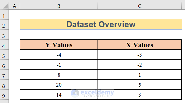
We have Y-values in Column B and X-values in Column C. The values for Y are obtained via linear equation.
Method 1 – Using the Excel INTERCEPT Function to Find Y Intercept
Steps:
- Insert the following formula in cell C11.
=INTERCEPT(B5:B9,C5:C9)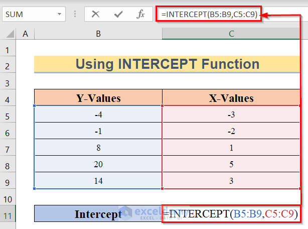
- Press the Enter button.
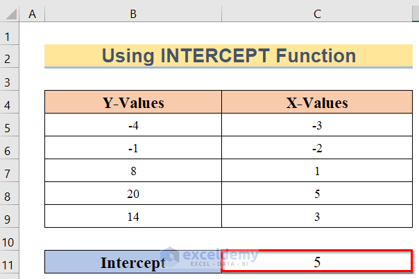
- You will get the y-intercept with the INTERCEPT function in Excel like the following image.
Method 2 – Excel AVERAGE and SLOPE Function to Find the Y Intercept
Steps:
- Insert the following formula in cell C11.
=AVERAGE(B5:B9)-SLOPE(B5:B9,C5:C9)*AVERAGE(C5:C9)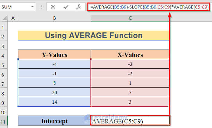
How Does the Formula Work?
- AVERAGE(B5:B9): In the first portion, we have used the AVERAGE function and in the function, we have taken the input from B5 to B9 The function will take the values from these cells and give us the average value accordingly.
- SLOPE(B5:B9, C5:C9): From this section, we will get an idea about the SLOPE function. The function takes the input in two sections. In the first section, we have inserted B5 to B9 cells which represent y-values and in the second portion, we have inserted C5 to C9 cells which represent x-values.
- AVERAGE(B5:B9)-SLOPE(B5:B9, C5:C9)*AVERAGE(C5:C9): This is the whole equation. At first, we have taken the average of cells B5 to B9. Then, used the SLOPE function from C5 to C9 cells and multiplied the result by the average of cells C5 to c9 Thus, your y-intercept function is ready.
- Hit the Enter button.
- You will get the y-intercept.
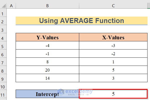
Read More: How to Find x-Intercept in Excel
Method 3 – Finding the Y Intercept by Using a Chart
Steps:
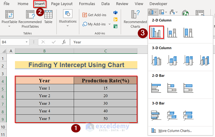
- We have Year in Column B and Production Rate (%) in column C.

- Go to Insert, then to Insert Column or Bar Chart, then select a 2-D column.
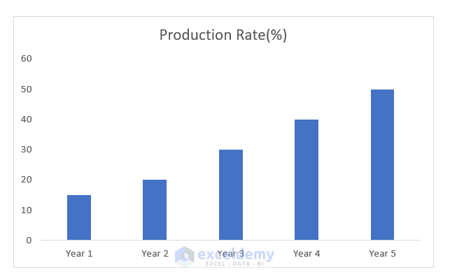
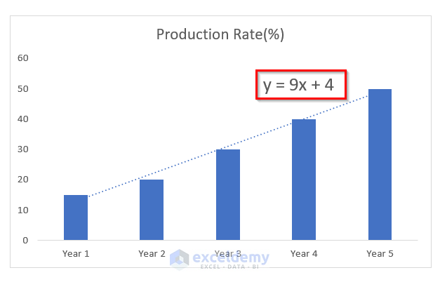
- You will get the column chart like the below image. We have the Production Rate (%) in the y-axis and the Year in the x-axis.
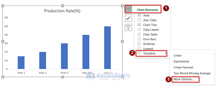
- Go to Chart Elements, check Trendline, and select More Options.
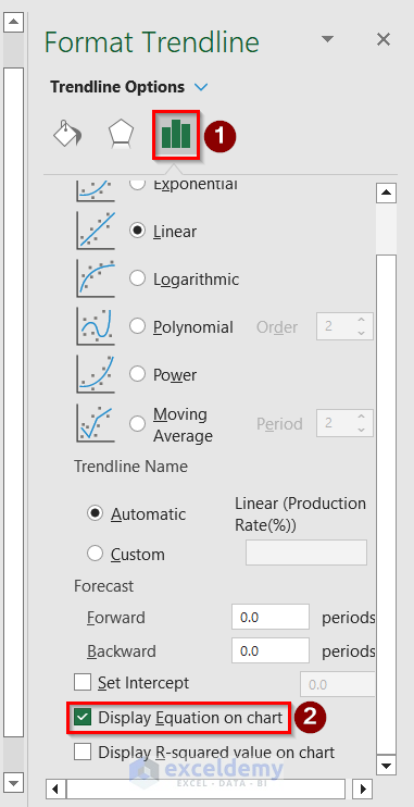
- In the Format Trendline window, go to Trendlines Options and select Display Equation on Chart option.
- We get the linear equation for this chart, y=9x+4. The value independent of x (i.e. the constant) is the y-intercept (in this case 4).
Read More: How to Set Intercept Trendline in Excel
How to Find the SLOPE in Excel
Steps:
- Y values are in B5:B9, and X values are in C5:C9.
- Insert the following formula in cell C11.
=SLOPE(B5:B9,C5:C9)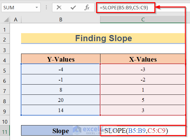
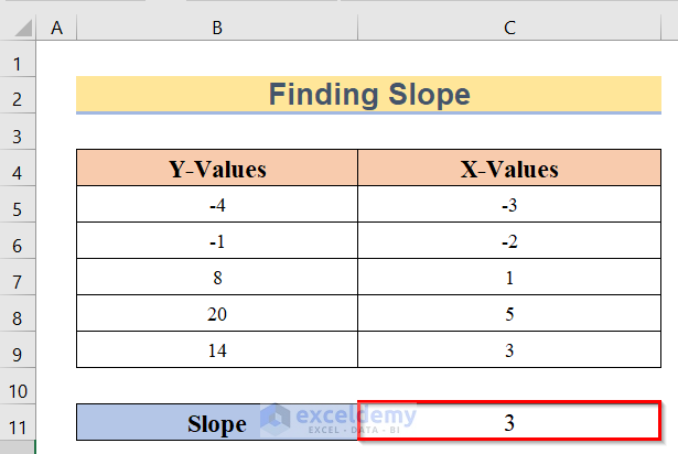
- Hit Enter.
Things to Remember
- The most important thing about using the INTERCEPT or SLOPE function is that you have to insert the y-values before the x-values.
Download the Practice Workbook
Related Articles
<< Go Back to Excel INTERCEPT Function | Excel Functions | Learn Excel
Get FREE Advanced Excel Exercises with Solutions!

