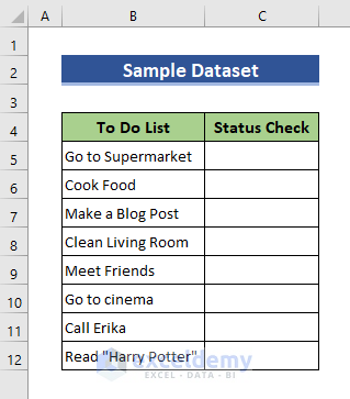
This is the sample dataset:
Step 1 – Enable the Developer Tab
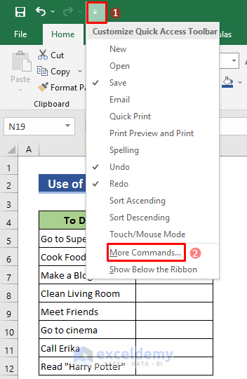
- Click Customize Quick Access Toolbar above the Home tab.
- Select More Commands.
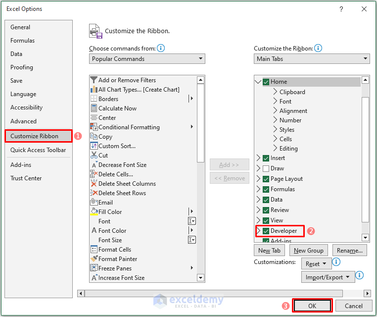
- In Customize Ribbon, check Developer.
- Click OK.
Read More: How to Make a Checklist in Excel Without Developer Tab
Step 2: Create Check Boxes
- Go to the Developer tab and click Insert.
- Click Check box.
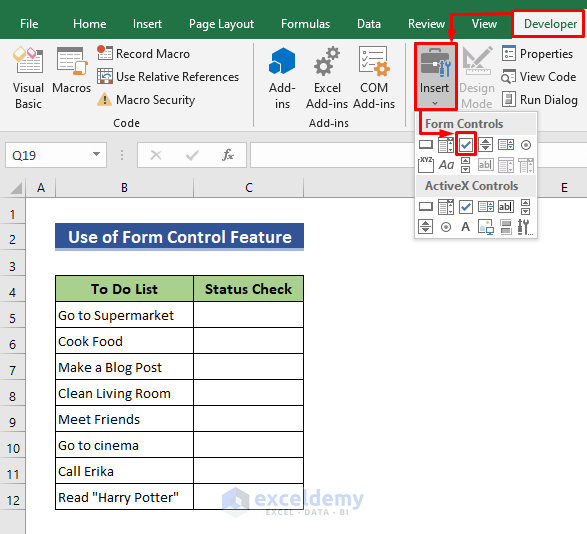
The cursor will display a “+” sign.
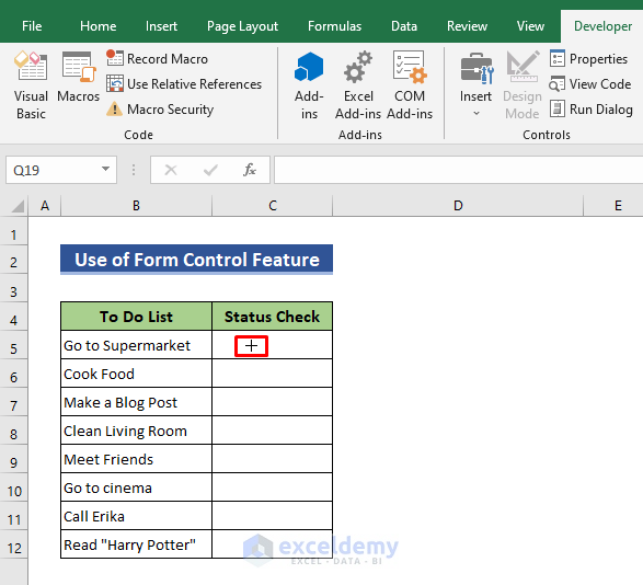
- Drag your cursor while holding the left button of the mouse to create a check box.
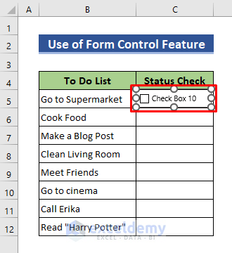
- To remove the text beside the check box, right-click and select Edit Text.
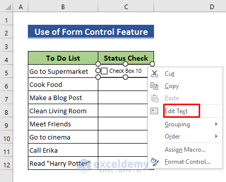
The Edit Text option is enabled.
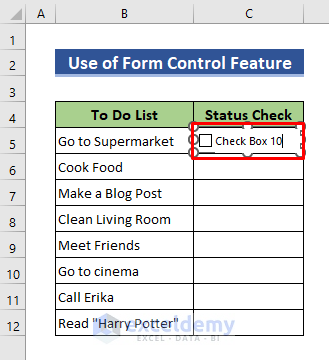
- Press Backspace to delete the text.
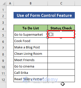
- Hold the left button of your mouse to move the check box and place it in the middle of the cell.
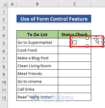
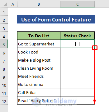
- Select the cell and drag the bottom right corner of the cell.
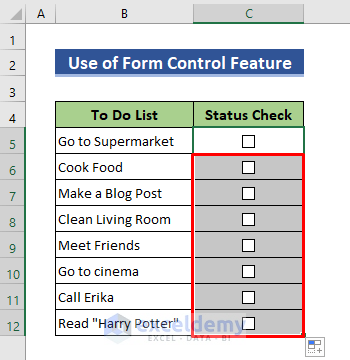
You will get check boxes in all cells.
Read More: How to Make a Daily Checklist in Excel
Step 3: Check the Boxes
- Move the cursor to the check box you want to check.
- The cursor will display a Hand Icon.
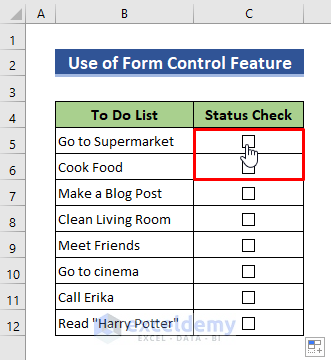
- Click the box to check it.
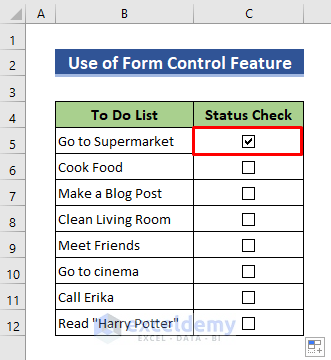
Read More: How to Create an Interactive Checklist in Excel
Step 4: Link Cells
To show “TRUE” or “FALSE” depending on the status of check boxes.
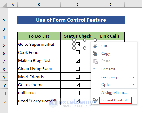
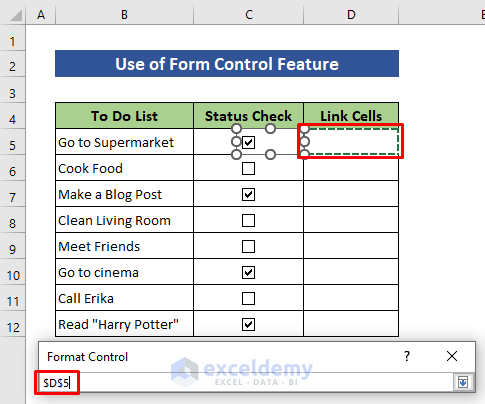
- Right-click the check box and select Format Control.
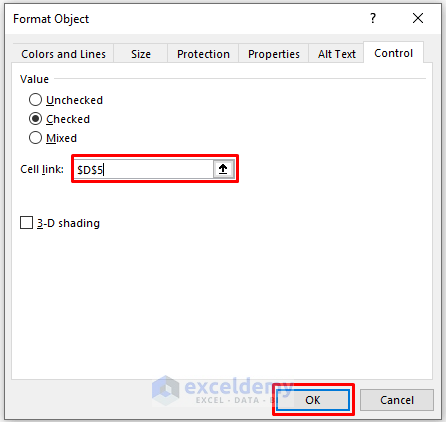
- Click the arrow in Cell link.
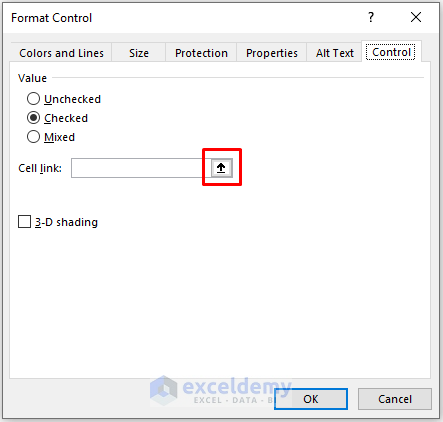
- Select the cell you want to link with the box. Here, D5.
- Press Enter.
- Click OK.
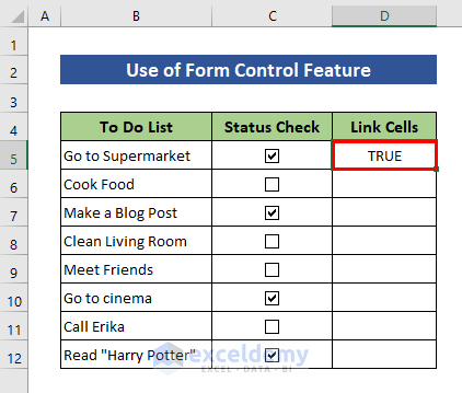
D5 is showing “TRUE”.
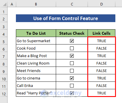
- Follow the same steps for the other cells.
Checked cells will show “TRUTH” and unchecked cells will show “FALSE”.
Step 5: Format the Checklist Color
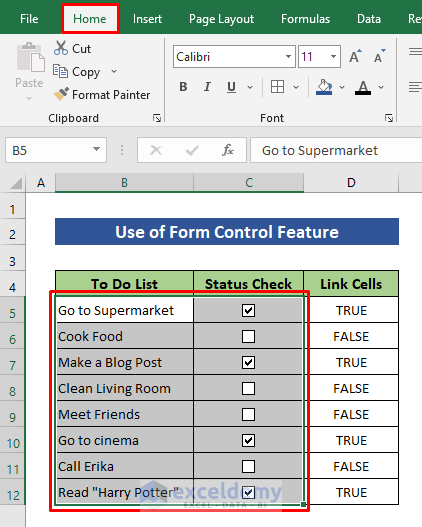
- Select the To Do List and Status Check columns.
- Go to the Home tab.
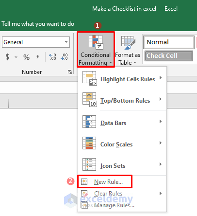
- Click Conditional Formatting and select New Rule.
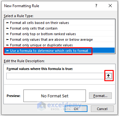
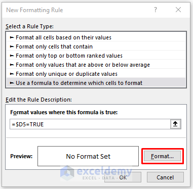
- Select Use a formula to determine which cells to format and click the upward arrow.
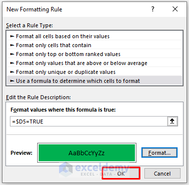
- Enter =$D5=TRUE in New Formatting Rule.
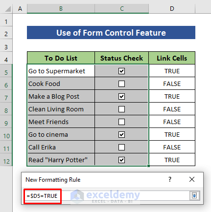
- Press Enter and click Format.
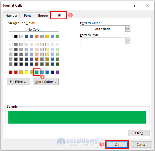
- Go to the Fill tab and choose a color.
- Click OK.
- Press Enter.
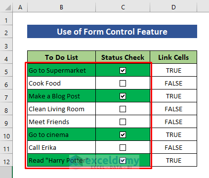
All rows with checked boxes display the selected color.
Read More: How to Make Checklist with Conditional Formatting in Excel
Download Practice Workbook
Download the practice workbook.


