We have a dataset of Payment Details of Customers.
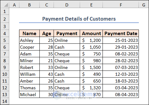
Note: This is a basic dataset to keep things simple. In a practical scenario, you may encounter a much larger and more complex dataset.
AND Function:
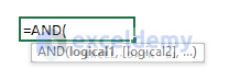
- Syntax:
=AND(logical1, [logical2])
- Arguments Explanation:
| Argument | Compulsory/Optional | Explanation |
|---|---|---|
| logical1 | Compulsory | 1st logical condition. |
| [logical2] | Optional | 2nd logical condition. |
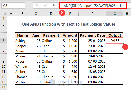
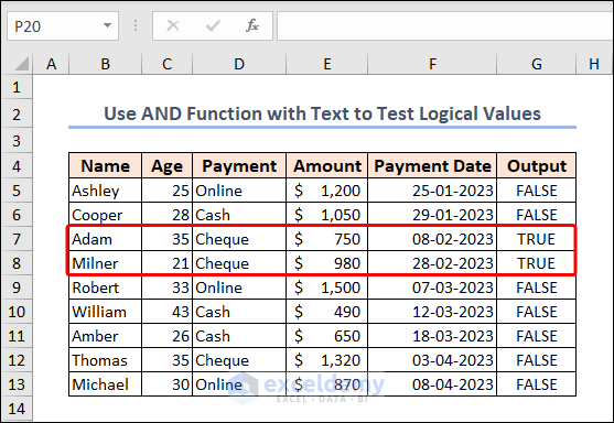
Example 1 – Use the AND Function with Text to Test Logical Values
Let’s find the transactions that have “Payment” via Cheque and the “Payment Date” is before April 1, 2023.
Steps:
- Create a new column where you can get the output/result. We named it “Output” under Column G.
- In the first cell of this column (cell G5), insert the following formula.
=AND(D5="Cheque",F5<DATE(2023,4,1))The first condition is that the value in cell D5 is equal to the text string “Cheque“. The second condition is that the date value in cell F5 is earlier than April 1st, 2023 (which is represented by the DATE function). The AND function is used to check if both of these conditions are true. If both conditions are true, the formula will return TRUE. If either condition is false, the formula will return FALSE.
- Get the results of the remaining cells in Column G by using the Fill Handle.
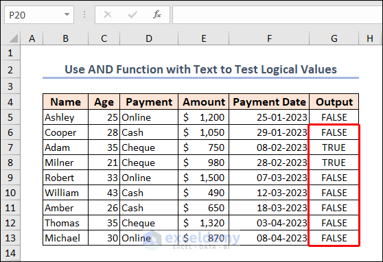
You can verify that Adam and Milner paid their bill by Cheque before the mentioned date. So, it returns TRUE in their case.
Read More: How to Return TRUE or FALSE Using Excel AND Function
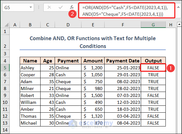
Example 2 – Combine AND and OR Functions with Text for Multiple Conditions in Excel
We’ll check if either of the two payment methods “Cash” or “Cheque” have a payment date that is before April 1st, 2023.
Steps:
- Paste the following formula in cell G5 and press Enter.
=OR(AND(D5="Cash",F5<DATE(2023,4,1)),AND(D5="Cheque",F5<DATE(2023,4,1)))Formula Breakdown
- AND(D5=”Cash”,F5<DATE(2023,4,1)): The first condition is that the value in cell D5 is equal to the text string “Cash” and the date value in cell F5 is earlier than April 1st, 2023.
- AND(D5=”Cheque”,F5<DATE(2023,4,1)): The second condition is that the value in cell D5 is equal to the text string “Cheque” and the date value in cell F5 is earlier than April 1st, 2023.
- OR(AND(D5=”Cash”,F5<DATE(2023,4,1)),AND(D5=”Cheque”,F5<DATE(2023,4,1))): The third condition is the combination of the first and second conditions joined by the OR function. This means that if either of the two conditions is true, the overall condition will be true.
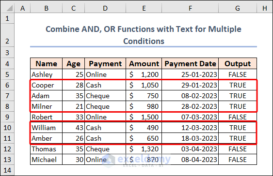
You can see that the highlighted rows have met these conditions (“Payment” and “Payment Date”), that’s why they got TRUE in the “Output” column.
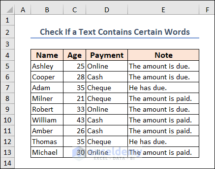
Example 3 – Check If a Text Contains Certain Words Using AND, ISNUMBER, and SEARCH Functions
In the “Note” column, we have the status of payment of the customers. We’ll check the transactions which have “amount” and “due” texts in Column E.
Steps:
- In the first cell (cell F5) of the “Output” column, use the following formula.
=AND(ISNUMBER(SEARCH("amount",E5)),ISNUMBER(SEARCH("due",E5)))Formula Breakdown
- SEARCH(“amount”,E5): The SEARCH function is used to search for the word “amount” in cell E5. If “amount” is found in cell E5, the function returns the position of the first character of “amount” in E5. If the text string is not found in E5, the function returns the #VALUE! error.
- ISNUMBER(SEARCH(“due”,E5)): The ISNUMBER function is used to check if the result of the SEARCH function for “amount” is a number. If the result is a number, the function returns TRUE. If the result is not a number, the function returns FALSE.
- The same process is repeated for the word “due”, using the SEARCH and ISNUMBER functions.
- AND(ISNUMBER(SEARCH(“amount”,E5)),ISNUMBER(SEARCH(“due”,E5))): Finally, the AND function is used to check if both of the previous conditions (i.e., “amount” and “due” are found in E5) are true. If both conditions are true, the AND function returns TRUE. If either condition is false, the AND function returns FALSE.
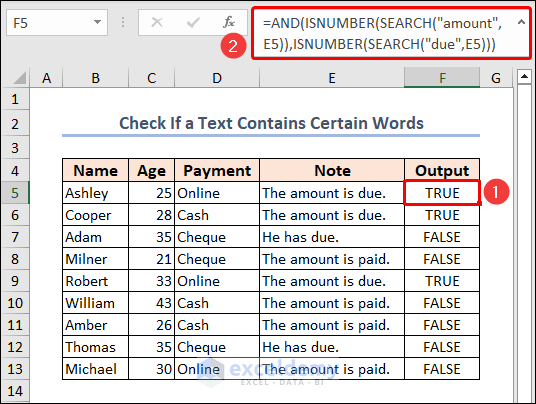
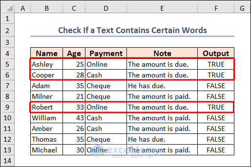
Rows 5, 6, and 9 got TRUE output as there are “amount” and “due” both texts present in the Note column.
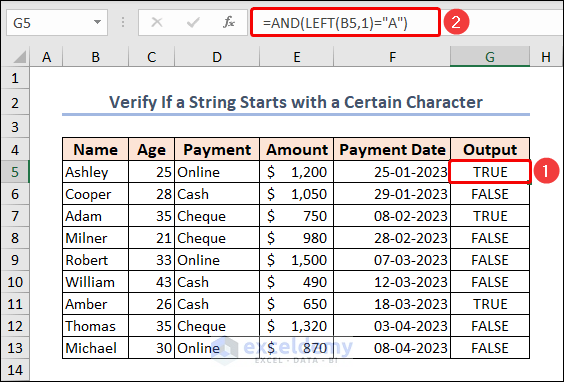
Example 4 – Verify If a String Starts with a Certain Character
We want to know which customer name starts with “A” in Column B.
Steps:
- In cell G5, use the following formula.
=AND(LEFT(B5,1)="A")Here, B5 represents the first customer name. The LEFT function is used to extract the first character of the text string in cell B5.
The = (equal) operator is used to compare the extracted character to the letter “A“. If the extracted character is equal to “A“, the = operator returns TRUE, otherwise returns FALSE. Since there is only one condition being checked in this formula, the AND function is not strictly necessary.
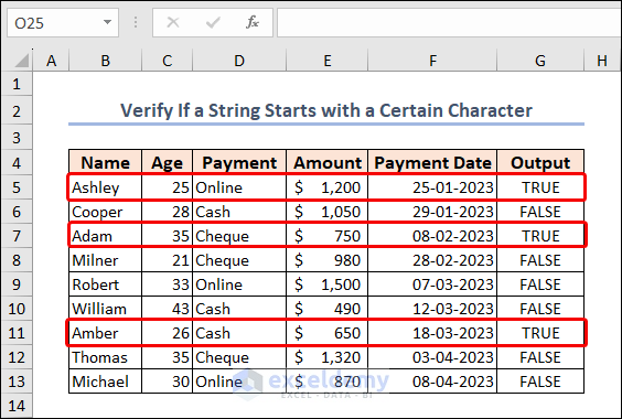
All TRUE rows have names that start with an “A”.
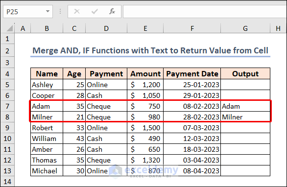
Example 5 – Merge AND and IF Functions with Text to Return a Value from a Cell in Excel
In Example 1, we got TRUE if both conditions are met. Here, we’ll get the name of the customer in the “Output” column if the same pair of conditions get fulfilled.
Steps:
- Paste the formula below in cell G5 and press Enter.
=IF(AND(D5="Cheque",F5<DATE(2023,4,1)),B5,"")If both conditions are true, the value in cell B5 will be returned by the IF function. If either condition is false, an empty string will be returned.

Excel returned only the names of Adam and Milner because their transactions fulfilled all the criteria.
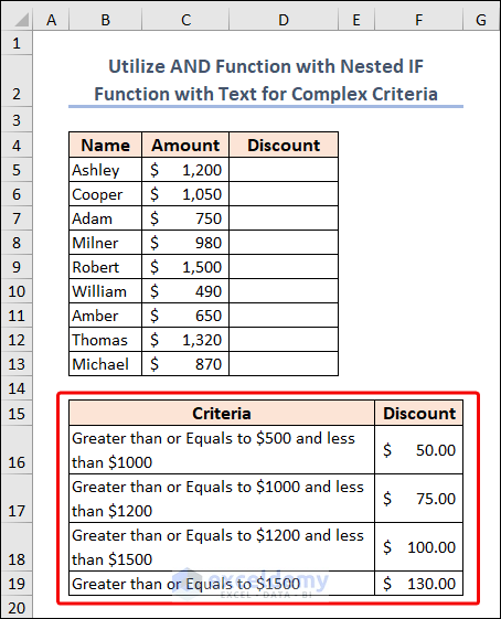
Example 6 – Utilize the AND Function with a Nested IF Function with Text for Complex Criteria in Excel
We want to give a discount based on the payment amount of each customer. The discount criteria and the corresponding amount is in the B15:F19 range in the image below. We’ll get the total discount for each customer.
Steps:
- Use the following formula in cell D5.
=IF(AND(C5>=1500),130,IF(AND(C5>=1200,C5<1500),100,IF(AND(C5>=1000,C5<1200),75,IF(AND(C5>=500,C5<1000),50,"Not Applied"))))Formula Breakdown
- IF(AND(C5>=1500): If the value in cell C5 is greater than or equal to 1500, then return the value 130.
- IF(AND(C5>=1200,C5<1500): If the value in cell C5 is between 1200 and 1499, then return the value 100.
- IF(AND(C5>=1000,C5<1200): If the value in cell C5 is between 1000 and 1199, then return the value 75.
- IF(AND(C5>=500,C5<1000): If the value in cell C5 is between 500 and 999, then return the value 50. Otherwise, return the text “Not Applied“.
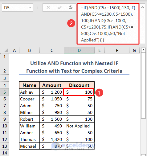
We got Not Applied in cell D10 because the amount is less than $500.
Example 7 – Use a Nested AND Function with Text to Evaluate Multiple Logical Conditions Simultaneously in Excel
We’ll determine if someone is eligible or not considering different criteria. The criteria are the Payment has to be in Cash, the Amount has to be above $900, the Payment Date has to be before April 1, 2023 and the Age of the customer has to be between or equal to 25 to 30.
Steps:
- Put the following formula in cell G5.
=IF(AND(D5="Cash",E5>900,F5<DATE(2023,4,1),AND(C5>=25,C5<=30)),"Yes","No")If all the conditions are true, the IF function will return Yes as the value_if_true argument. Otherwise, it returns No.
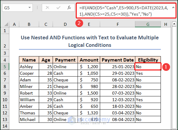
You can see Cooper and William have cracked the code only.
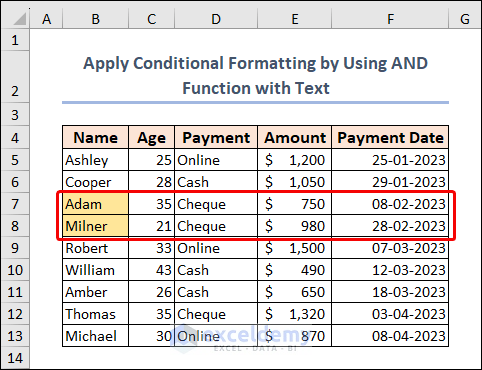
Example 8 – Apply Conditional Formatting by Using the AND Function with Text
Steps:
- Select cells (B5:B13) where you want to apply the Conditional Formatting rules.
- Choose the New Rule from the Conditional Formatting drop-down.
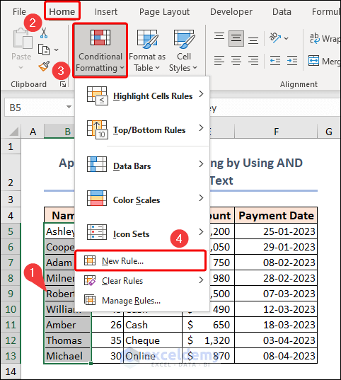
- A new dialog box will appear named New Formatting Rule.
- Select the Use a formula to determine which cells to format option.
- In the Format values where this formula is true box, put the following formula:
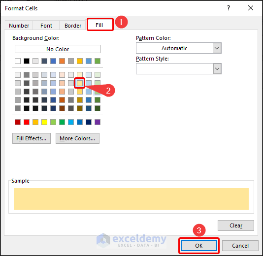
=AND(D5="Cheque",F5<DATE(2023,4,1))- Click Format.
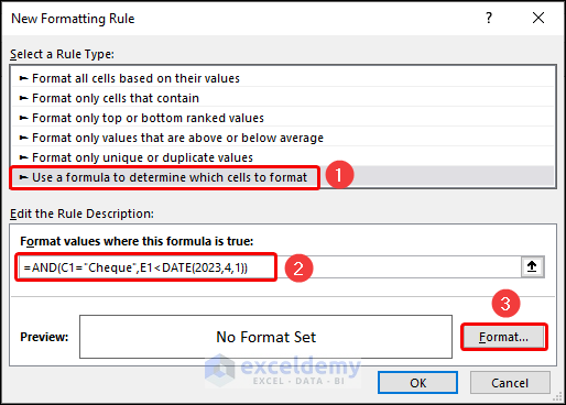
- Go to the Fill tab and select a desired color from the list, then press OK.
- Press OK to get the results.
Read More: How to Use IF with AND Function in Excel
Limitations of Using AND Function with Text Values in Excel
- Starting from Excel 2007, the AND function has the capability to test up to 255 arguments, as long as the overall length of the formula does not go beyond 8,162 characters.
- The AND function will produce a #VALUE! error under two conditions: if any of the logical conditions are passed as text, or if none of the arguments result in a logical value.
- If all of the arguments provided in the AND function are empty cells, the function will return a #VALUE! error.
- The AND function in Excel does not differentiate between uppercase and lowercase letters, which means it is not case-sensitive. This means that when you use the AND function to evaluate logical tests or conditions, it will treat uppercase and lowercase letters as the same. For example, “TRUE” and “true” will be evaluated as equivalent by the AND function.
- Unlike some other Excel functions, such as COUNTIF or SUMIF, the AND function does not support the use of wildcards. This means that users cannot use special characters such as asterisks (*) or question marks (?) as part of the arguments to the AND function in order to match a wider range of values. Instead, users must specify exact criteria for each argument in order to use the AND function effectively.
Things to Remember
- When using the AND function with text, enclose each condition in quotation marks.
- You can combine this function with other Excel functions, such as IF and COUNTIF, to create more complex formulas.
- Be careful when using the AND function with a large number of conditions, as it can become unwieldy and difficult to manage.
Frequently Asked Questions
How do I use the AND function with text in Excel?
To use the AND function with text in Excel, you need to enter each condition as a separate argument within the function, enclosed in quotation marks.
Can I use wildcards with the AND function in Excel?
No. It doesn’t support wildcards like asterisks (*) or question marks (?) to search for partial matches in text.
How many conditions can I use with the AND function in Excel?
You can use up to 255 conditions with the AND function in Excel.
How can I check if any of the conditions are false with the AND function in Excel?
You can use the NOT function in combination with the AND function to check if any of the conditions are false, rather than all of them being true.
Download the Practice File
You may download the following Excel workbook for better understanding and practice yourself.
Related Articles
- How to Use IFS and AND Functions Together in Excel
- Nested IF and AND Functions in Excel
- How to Use SUMIF and AND Function in Excel
<< Go Back to Excel AND Function | Excel Functions | Learn Excel
Get FREE Advanced Excel Exercises with Solutions!
