This article is intended for beginner users of Excel. We will discuss the basics of how to use Microsoft Excel and describe how to do 25 of the most common tasks. The methods we use are compatible with Microsoft Excel 2007, 2013, 2016, 2019, 365 and later.
How to Create a Blank Microsoft Excel Workbook
Let’s start right at the beginning, by creating a new Microsoft Excel workbook. This can be done either from within an existing workbook or directly from Windows.
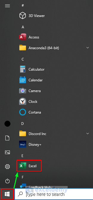
Directly from Windows:
- Click on the Start button on the Desktop Taskbar.
- Click the Excel icon from the list of installed applications.
From an Existing Workbook:
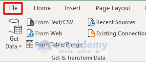
- Click on the File tab.
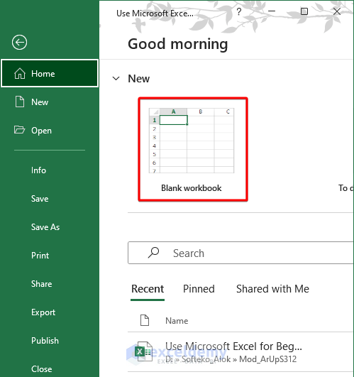
- Click on the Blank workbook option.
Keyboard Shortcut:
Just press Ctrl+N from inside an existing workbook and a new workbook will open.
Introduction to Excel Tabs / Ribbons: Home, Insert, Formulas, Data, Etc.
Excel’s Tabs or Ribbons are located at the top of every worksheet in an Excel workbook.
This section contains all the tools available in Excel.

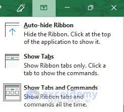
We can customize this section from the Ribbon Display Options.
The Home Tab:
The Home tab contains all the basic features to make an Excel file, such as font, size, color, border, background color, alignment, number format, etc. It also contains cell height, width, sort, filter, find & replace, and other features.
The Insert Tab:
The Insert tab contains lots of features, mainly concerning the insertion of images, text boxes, equations, symbols, etc.
The Formulas Tab:
The Formulas tab is where the different types of formulas used in Excel are located. Formulas are made from Excel Functions. Below, we will discuss different functions, Evaluate Formula and the Name Manager.
Excel Data Tab:
The Data tab houses the features related to data customization, such as forming tables, grouping & ungrouping data, data validation, consolidating, flash fill, etc.
How to Use Microsoft Excel for Beginners: 25 Common Tasks
Though Microsoft Excel has many advanced functions, even a built-in coding language, we will cover some of the most common tasks for beginners here.
Method 1 – Customize the Row and Column Format of an Excel Workbook
We can customize the format of cells to present our data more effectively.
Steps:
- Move the cursor to the upper leftmost corner of the dataset.
- In the Home tab, click on Format from the Cells tab drop-down.
- Click on the Row Height option from the Format drop-down list.
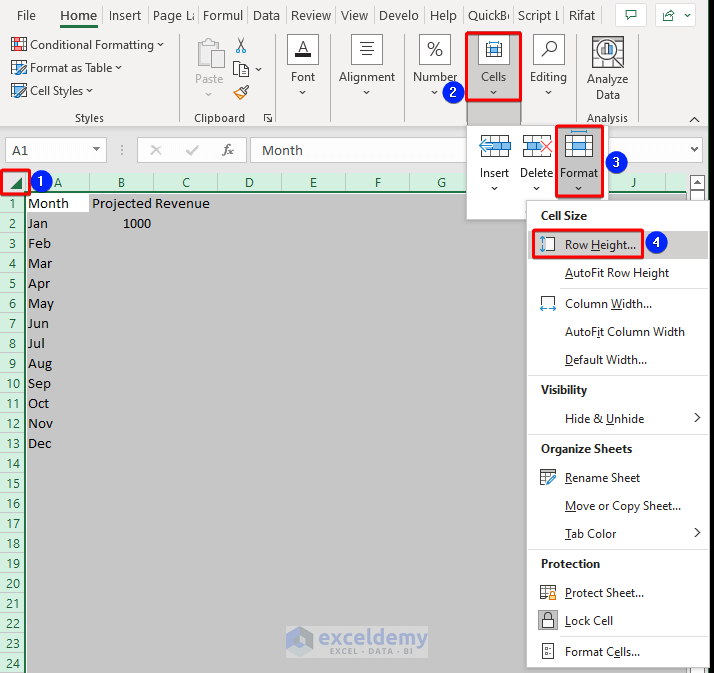
The Row Height window appears.
- Input the Row height and press the OK button.

The cell height has been changed. But the data of Cell B1 doesn’t fit in the cell well, so we’ll adjust the width of this cell.
- Place the cursor at the border of columns B and C.
- Double-click the mouse left button.
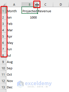
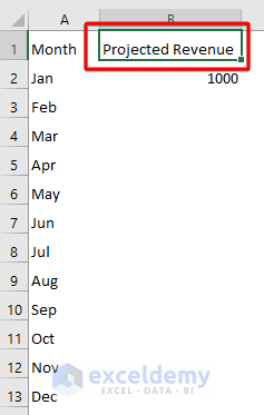
The data now fits well in the auto-adjusted column width.
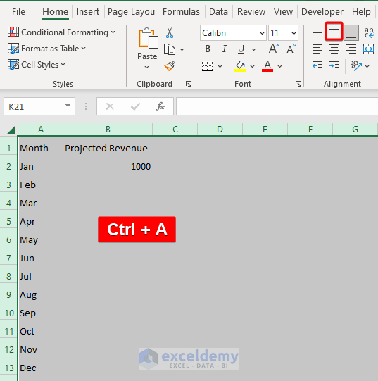
- Select the whole dataset by pressing Ctrl + A.
- Choose the Middle option from the Alignment section.
We can also set the borders of each cell:
- Select the cells to which you want to add borders..
- Go to the Borders drop-down.
- Select the All Borders option from the drop-down list.
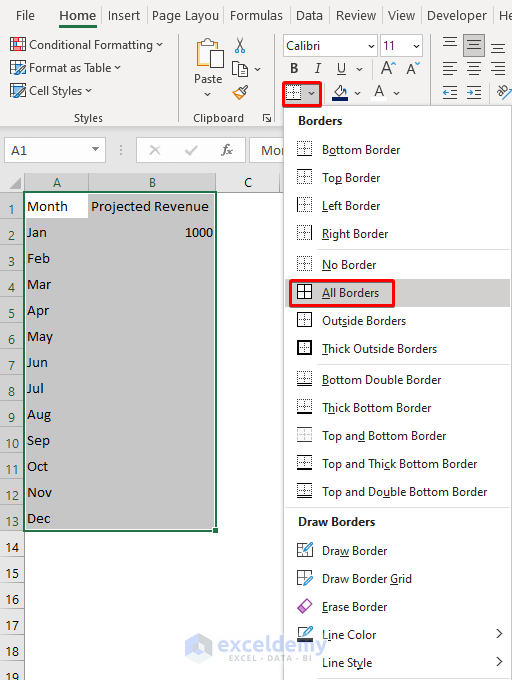
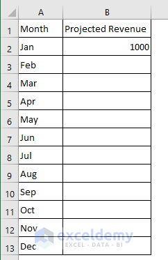
The cells with borders stand out from the rest of the sheet.
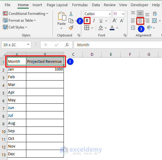
Let’s change the format of the headings of both columns.
- Select the Range A1:B1.
- Select B for bold from the Font section.
- Click on Center from the Alignment section.
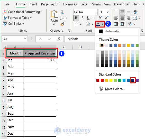
Now, we will change the font and background color of those cells.
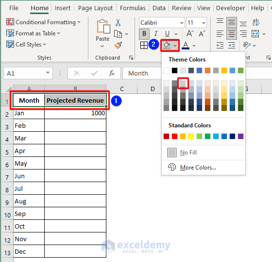
Both options are located in the Font section.
Method 2 – How to Apply a Number Format and Increase/Decrease Decimal Places in Excel
Microsoft Excel has different number formats for various purposes: Number, Currency, Date, Percentage, etc. Let’s go through how to find and apply these options in the Microsoft Excel UI.
Steps:
First, let’s choose a cell format from the Number section of the Home tab.

- Click on the drop-down list.

A list of formats are offered.
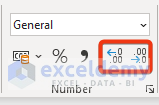
We can also add decimal points, and increase or decrease the number of digits.
Example:
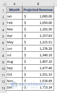
Suppose we want the values showing in the Projected Revenue column to be in a certain currency with a specific number of decimal points.
Steps:
- Select the Range B2:B13.
- Press Ctrl +1.
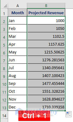
The Format Cells window appears.
- Choose Accounting from the Number tab.
- Choose the currency from the Symbol drop-down list.
- Set the Decimal places.
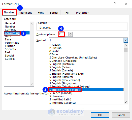
- Click the OK button.
Method 3 – Use Conditional Formatting to Analyze Data for Specified Criteria
Using the Conditional Formatting feature, we can apply formats to specific cells based on different conditions like the highest value, lowest value, etc. We can also insert formulas to set criteria in conditional formatting.
The Conditional Formatting feature is available in the Home tab.
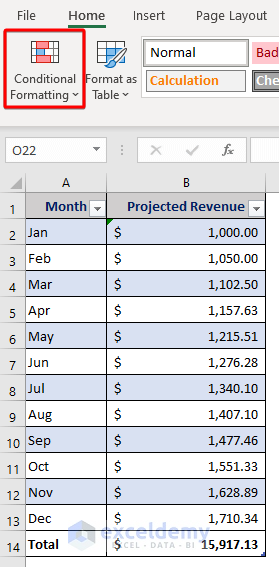
Suppose we want to highlight the cells of the dataset between two values.
Steps:
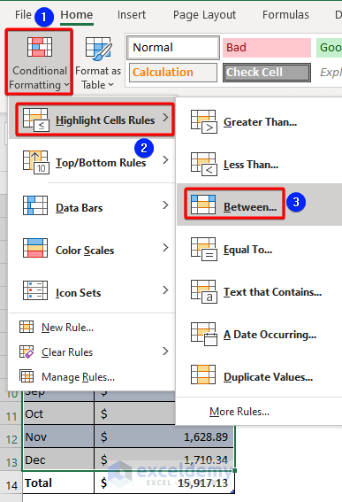
- Select the data to be conditionally formatted using the mouse.
- Click on the Conditional Formatting button.
- Choose the Between option from the Highlight Cells Rules.
A dialog box opens.
- Insert 1200 as the lowest and 1450 as the highest value.
- Select a highlighting color from the drop-down list.
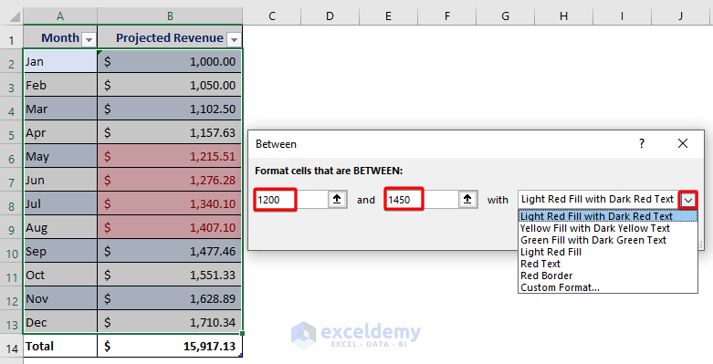
Cells B6:B9 are highlighted with a light red color.
Method 4 – How to Create, Design, and Use an Excel Table
Turning a range of cells into a Table has many advantages, like the ability to filter and sort. We can form a table from the Insert ribbon or by using a keyboard shortcut.
Steps:
- Select the whole dataset (or some cells inside the data).
- Go to the Insert tab and click on the Table option.
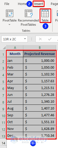
We can also do this by pressing Ctrl + T.
The Create Table dialog box opens.
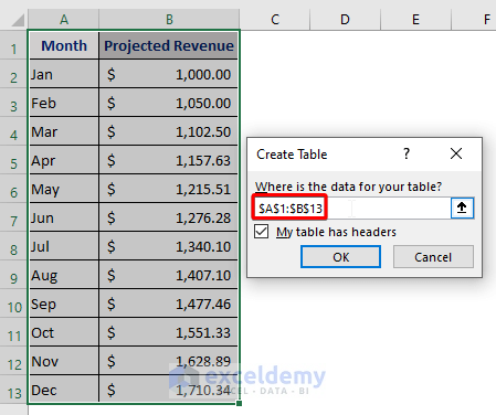
Our selected range is shown here.
- Mark the My table has headers option.
- Click OK.
The name of the Table appears on the upper left side of the ribbon.
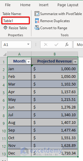
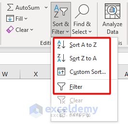
Now, there is a drop-down symbol next to the header in each column of the table. We can avail ourselves of the Filter and Sort features here.
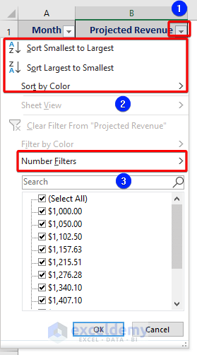
- We can also access the Sort and Filter options from the Editing section of the Home tab.
Excel Tables have a dedicated tab named Table Design in the ribbon that will appear when a table is selected.

The Table Design tab has some features to make tables more visually appealing and informative.
For example, we can easily get the total amount of a column by checking Total Row.
- Just tick the Total Row option from the Table Style Options section.
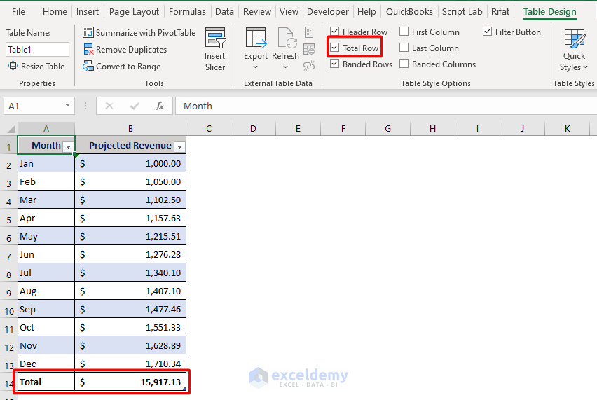
There is a new addition to the dataset. The Total row shows the sum of the rows above.
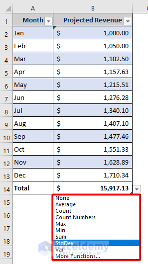
We can also apply other options to the Total row.
- Click on the drop-down button of this Total row, and more options like average, count, max, min, etc. are available.
Method 5 – Copying and Pasting in Excel
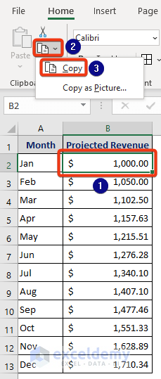
We can copy and paste from the Home tab.
Steps:
- Move the cursor to cell B2.
- Click on the drop-down list in the Copy section of the Home tab.
- Select Copy.
We can also press the usual Ctrl + C keyboard shortcut.
- Click on the Paste option.
A list of options is displayed.
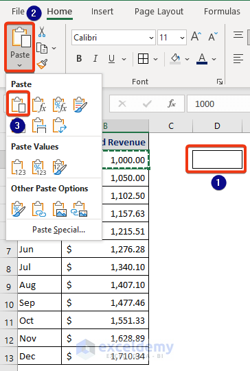
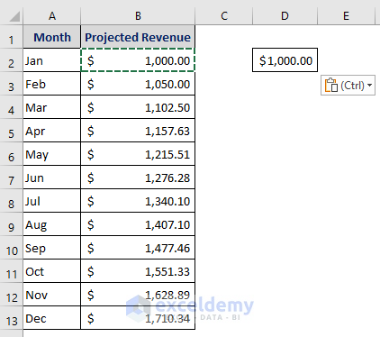
The copied data has been pasted in the dataset.
Method 6 – Applying Excel Fonts, Font Size, Font Color, Fill Color, Borders, and Others Commands
Now let’s see how to customize the font section. We can choose the font type, size, style, color, background color, and more.
Steps:
- Click on the arrow in the Font section.
The Format Cells window opens on the Font tab.
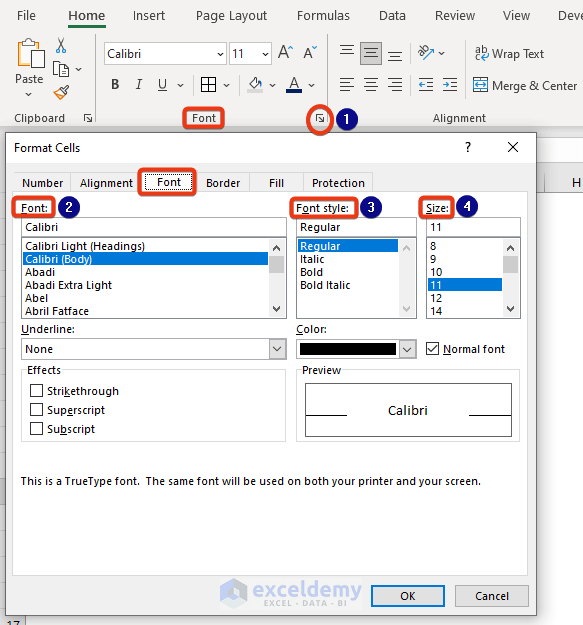
We can also open it with the keyboard shortcut Ctrl+ Shift+ F.
Method 7 – How to Insert or Delete Cells, Rows, Columns, and Sheets in Excel
Steps:
The Insert and Delete options are located in the Cells section of the Home tab.

- Click on the drop-down of Insert.
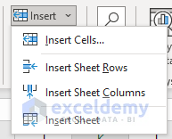
There are options for inserting cells, rows, columns, and sheets.
Similar options are to be found in the Delete section.
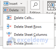
These operations can also be accessed from the Context Menu:
- Click on any row, column or cell and then press the right button of the mouse.

The Insert and Delete options appear in the list.
Another way to insert a new sheet:
- Go to the bottom section of the worksheet and click on the plus button.
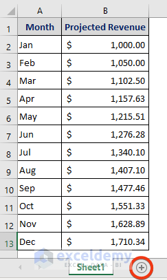
A new worksheet will be inserted.
Method 8 – Using the Find & Select Feature in Excel
Another useful feature in the Home tab is the Find & Select feature,
Steps:
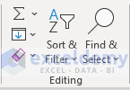
- Click on the Find & Select drop-down.
- Select either the Find or Replace option.
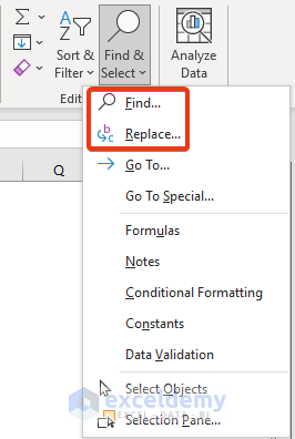
The Replace option will search for any value and replace it.
- Click on either Find or Replace and the Find & Replace box below will appear.
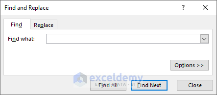
- Input anything in the Find what box.
We can also press Ctrl + F as the keyboard shortcut to open Find and Replace. To go to Replace directly, press Ctrl+H.
Method 9 – How to Easily Create a Chart in Microsoft Excel
Now let’s create a chart in Excel.
Steps:
- Select the dataset without the total row.
- Click on the Insert tab.
- Click on the arrow button in the Charts section.
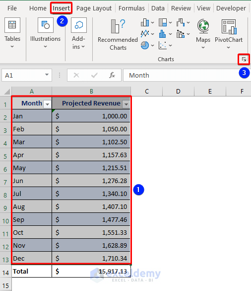
The Insert Chart window appears.
- Go to All Charts and select a chart.
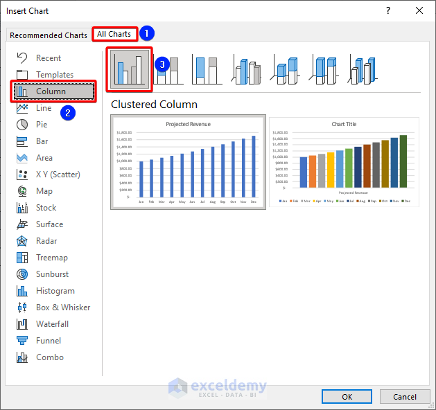
- Click OK.
A chart appears alongside the dataset.
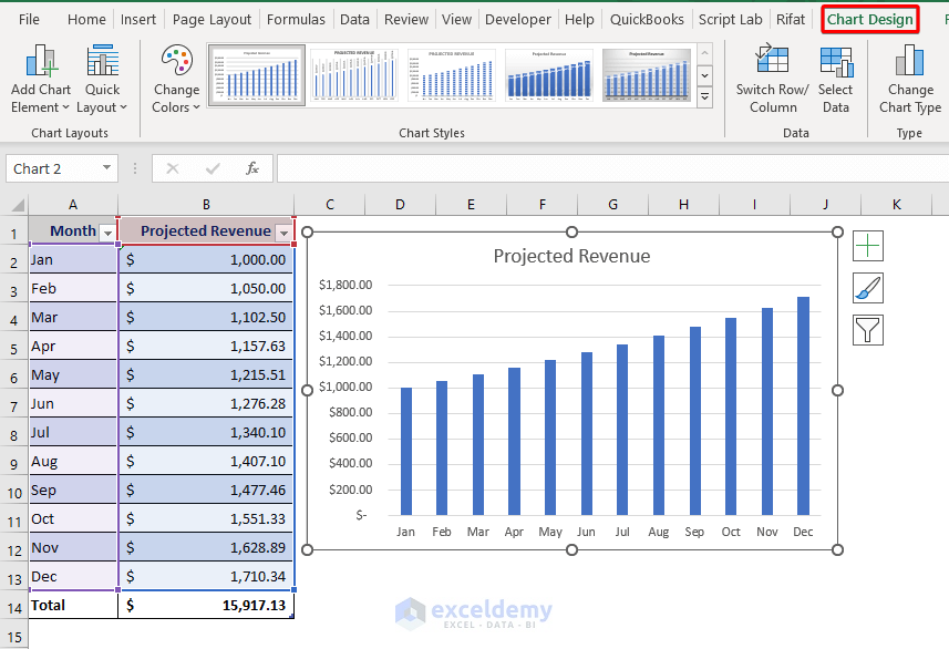
We can customize the chart using the dedicated tab named Chart Design which will appear on the ribbon when a chart is selected in the worksheet
Method 10 – Adding Images or Shapes Using the Illustration Feature of the Insert Tab
From the Illustration section, we can insert images, shapes, screenshots, etc.
Steps:
- Go to Insert >> Illustration.
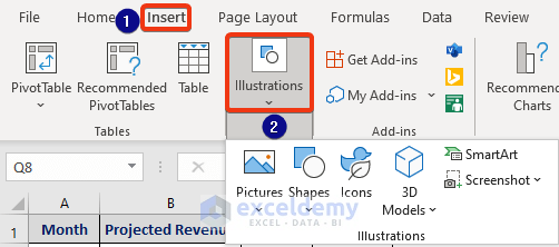
There are different options available here.
- Click on the Picture drop-down to insert a picture.
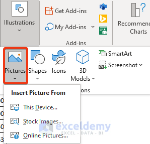
Different source references from which to insert the image are offered.
- Click on the Shapes drop-down to insert any of the many available shapes.
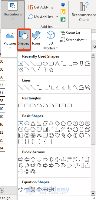
There are also other options, but for the sake of brevity we’ll leave those for you to explore.
Method 11 – How to Add Text Boxes in an Excel Sheet
Now, we will introduce the Text box feature, available on the Insert tab.
Let’s add a text box.
Steps:
- Go to Insert >> Text.

- Click on the drop-down symbol.
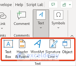
A list with different options opens.
- Click on the Text Box field and a rectangular box will appear.
- Place that box where you want it on the worksheet.
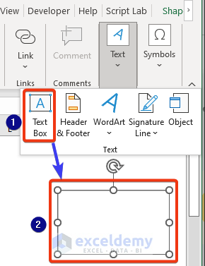
- Resize the rectangular box as you like.
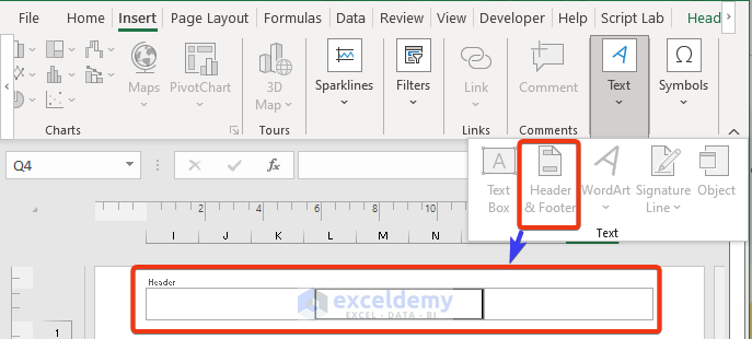
Another feature is Header & Footer.
The Footer is usually used to present the page number at the bottom of each page. On the other hand, a Header is used to present any text common to all the pages.
- To make use of this feature, click on the Header & Footer section on the Insert tab.
Method 12 – Inserting Equations and Symbols in Microsoft Excel
The Equation and Symbol features are sub-sections of the Symbols field.
Steps:
- Go to Insert >> Symbols.
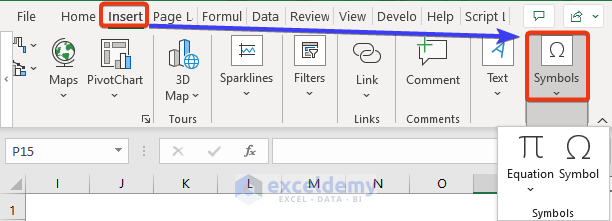
- Click on the Equation drop-down.
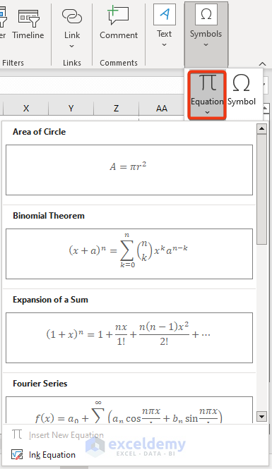
We get a set of equations.
To insert a symbol:
- Click on the Symbol section.
A new window named Symbol opens.
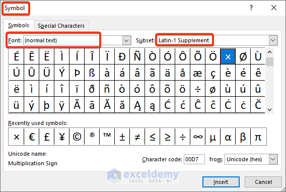
- Select your desired symbol and click Insert to insert it into the active cell.
Method 13 – Some of the Most Commonly Used Excel Functions
Excel functions are arguably the most useful feature of this feature-packed software. A vast selection of built-in functions are available which can be used alone or in combination with other functions and features. Here are a few of the most commonly used functions in Excel.
- SUM – Returns the sum of a series or a range of numbers.
- AVERAGE – Returns the average of a series.
- IF – This is a conditional function. If the condition is met one value is returned, otherwise optionally another is returned..
- MIN – Determines the smallest number of a range.
- MAX – Determines the largest number of a range.
- COUNT – Counts the number of cells in a selected range.
- COUNTA – Counts all the cells from a selection including error and blank cells.
- COUNTBLANK – Counts all the blank cells in a selection.
- LEN– Counts the number of characters in a cell.
- TRIM – Removes unnecessary spaces between strings.
- PRODUCT – Used to multiply numbers.
Microsoft Excel 365 version has more than 450 functions.
Method 14 – How to Evaluate a Formula in Excel
When you use a formula in Excel collected from an external source, or you have created a formula but it’s returning erroneous values, you may want to investigate what is wrong with that formula. For this purpose, Excel provides an Evaluate Formula option in the Formula Auditing section of the Formulas tab.
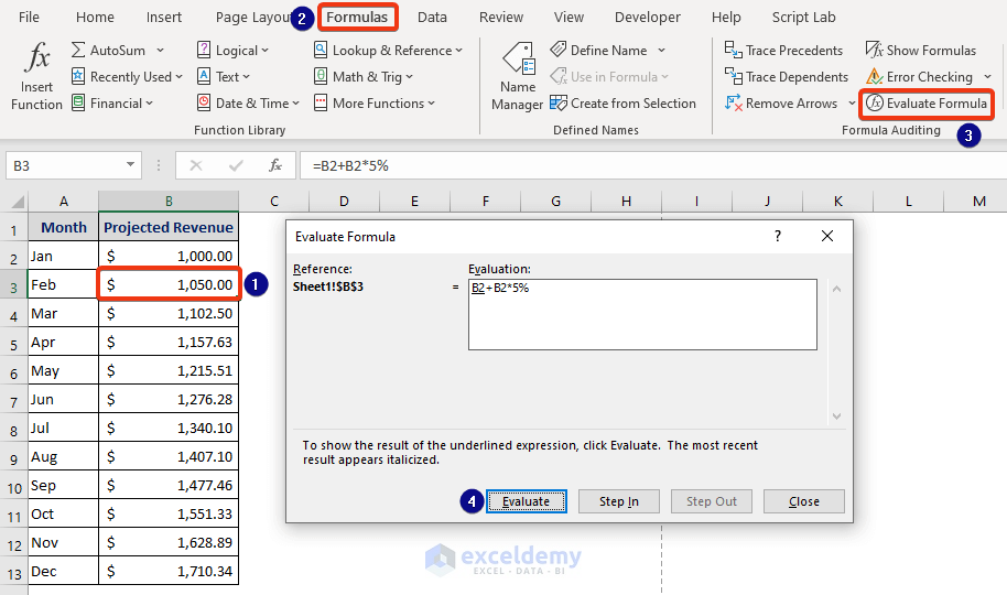
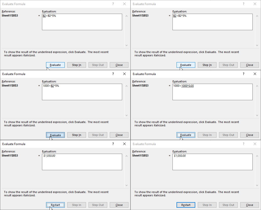
It will show the steps of how a formula works.
- Just click on the Evaluate button repeatedly and check the steps of your formula consecutively.
Method 15 – How to Define Names for a Range and Use Them in a Formula
This is debatably more advanced use of Excel than beginner level, but it is really useful to define a name for a range of cells, then use the name in formulas instead of the cell range.
Name Manager is one feature that can be used to group and name multiple related cells.
Steps:
- Select a range of cells.
- Choose Name Manager from the Formulas tab.
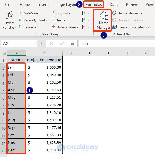
The Name Manager window appears.
- Click on the New option.
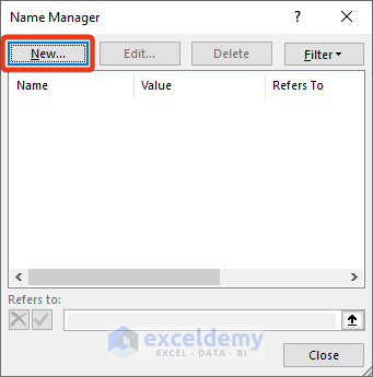
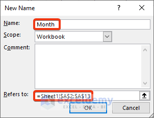
The selected range should be pre-selected in the refers to box.
- Enter a name in the Name box.
- Click the OK button.
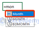
- Move the cursor to any cell and write ‘=mon‘.
A suggestion list opens.
- Choose the marked Month option.
- Press Enter.

In the dataset, we now have the names of all the months.
Method 16 – How to Create a List with Data Validation
In this section, we will discuss Data Validation. This feature will add a drop-down list from which we can select the value to be input into a cell, instead of typing it as usual. This allows input values to be controlled and validated.
Let’s add a drop-down list to select the month.
Steps:
- Add new cells for applying data validation as follows.
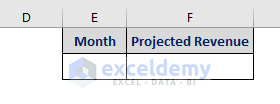
In the Month column, we will select the month value and the adjacent cell will show the Projected Revenue for the selected month.
- Select cell E2.
- Go to the Data Validation option on the Data tab.
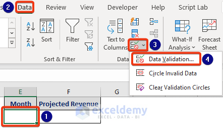
A new window named Data Validation appears.
- Choose List from the Allow field.
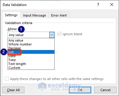
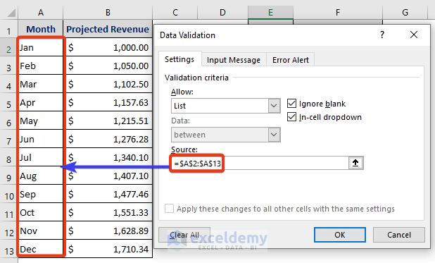
- Select the range of months in the Source field.
- Click OK.
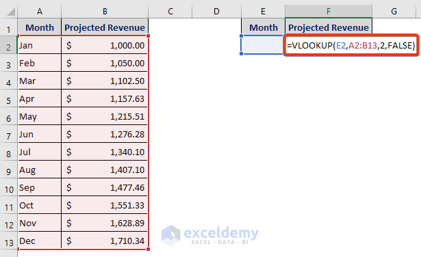
- Put the following formula based on the VLOOKUP function in cell F2:
=VLOOKUP(H2,A2:B13,2,FALSE)
- Click on the drop-down symbol for selecting Month.
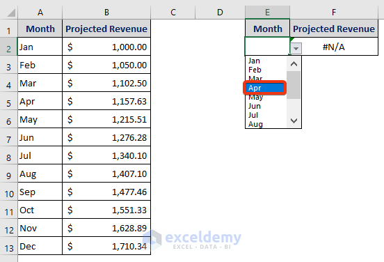
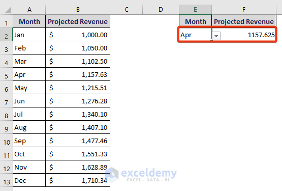
The revenue for the selected month from the drop-down list is showing in cell F2.
Method 17 – How to Consolidate Data in Microsoft Excel
We can combine data from different sheets or workbooks into a single sheet. Here, we will consolidate data by applying the Data Consolidation feature of the Data tab.
Steps:
Suppose we have data in 2 sheets, one for 2021 and another one for 2022. In the third sheet will combine those sheets.
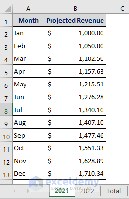
Worth mentioned is that in both of the sheets data starts from the same location. In the consolidation sheet, data will also be in the same location.
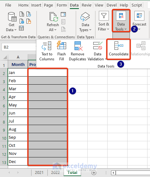
- Move the cursor to cell B2 and click on the Consolidate feature of the Data Tools.
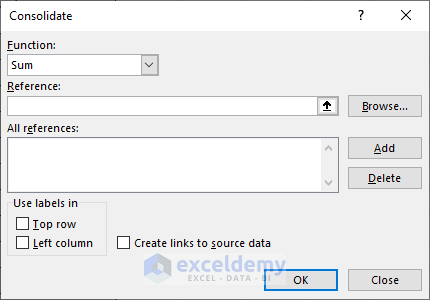
The Consolidate window will appear.
- Choose the SUM operation from the Function field.
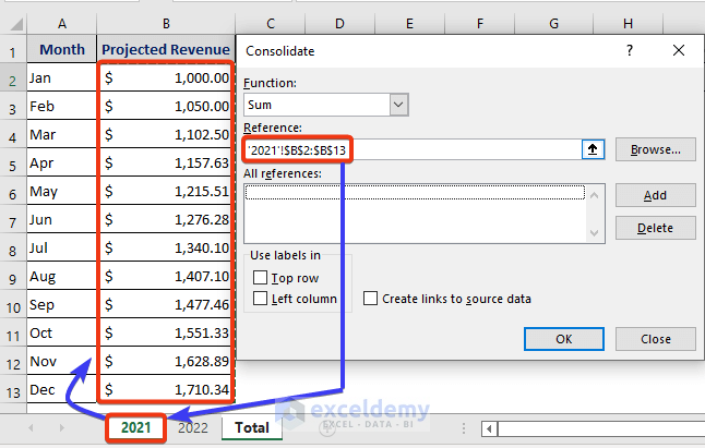
- Go to the Reference field.
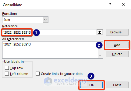
- Choose the desired cells from the sheet 2021. Then press the Add button.
- Select the range from sheet 2022.
- Click OK.
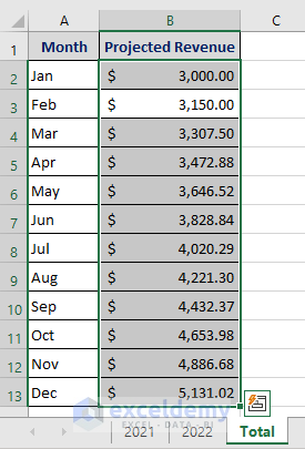
The consolidated total is displayed in the 3rd sheet.
Method 18 – How to Check Spelling and Get Workbook Data Statistics from the Review Tab
After typing lots of words, it’s hard and not particularly feasible to check the typing mistakes manually! Using the Spelling command, we can easily do a spell-check. It’s available in the Review tab.
There are several options in the Review tab. Of them, Spelling and Workbook Statistics are the most commonly used.

Steps:
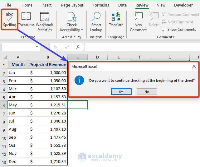
The Spelling feature checks the whole worksheet.
- Click on the Spelling command.
A dialog box will appear requesting permission.
- Choose Yes.
You can also access this feature by pressing F7 .
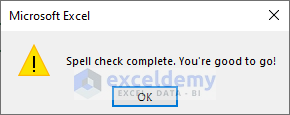
- Another dialog box will show the status of the spell-check.
Now, we will check the Worksheet Statistics.
- Click on that button.
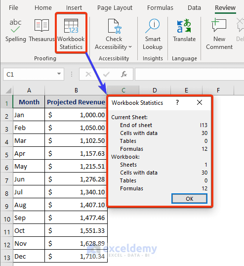
A window appears showing information on the worksheet: last data cell, how many cells have data, number of tables, number of formulas used, number of sheets, and more.
Method 19 – Using the View Ribbon
The View tab contains features to control how the worksheet looks. Let’s have a look at the most commonly used features of the View tab: Show, Zoom, and Freeze Panes.

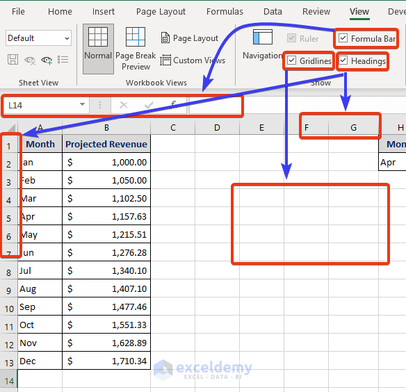
The Show section determines how a datasheet will look.
Tick or untick these features to enable/disable their display in your workbook:
- The Formula Bar shows the formula bar, including the Name Box.
- The Heading feature shows the row and column headings.
- The Gridlines option shows the gridlines of the worksheet.
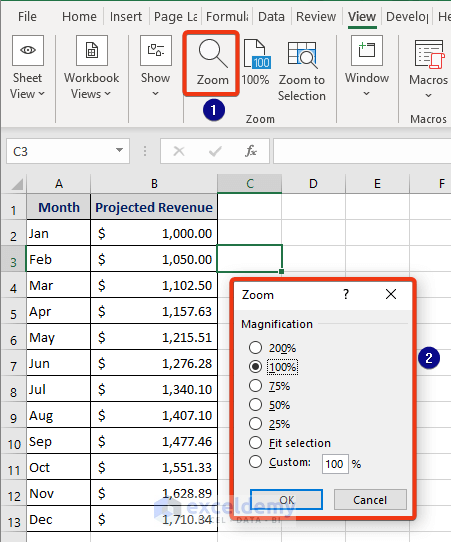
The Zoom feature is used for zooming in or out.
- Go to View >> Zoom.
A dialog box appears to set the zoom level.
- Tick the desired zoom level, then click OK.
Sometimes we need some rows and/or columns to remain visible constantly while we scroll through a large dataset. We can freeze parts of the sheet with the Freeze Panes option.
There are three options for freezing:
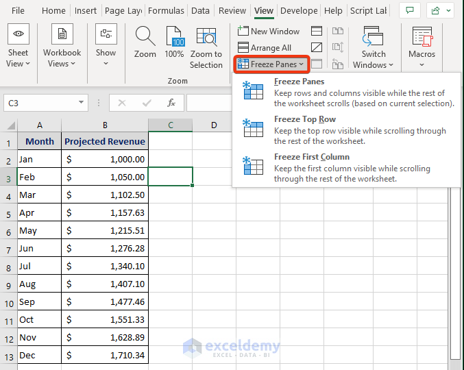
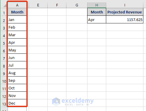
- To freeze the 1st column of the datasheet, select the Freeze First Column option.
The 1st column has been fixed.
The other options work similarly, freezing the top row or the cells above and to the left of a selected cell respectively.
Method 20 – How to Change the Selection Direction After Pressing the Enter Key
We can change the direction of the moving selection too.
- Press Alt+F+T to open the Excel Options window.
- Go to the Advanced option and select the direction you want.
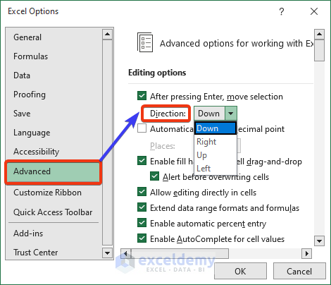
After pressing ENTER, the cursor will now jump to the next cell in the direction just specified.
Method 21 – How to Fill Data in a Column Using the Fill Handle
The Fill Handle saves having to copy the same formula or series across a range of cells manually.
We will apply the Fill Handle feature on cell A2. Suppose in Column A we want to fill the short names of the months in the cells below Jan.
Steps:
The Fill Handle icon will appear when you hover with your mouse over the bottom right corner of a cell, here cell A2.
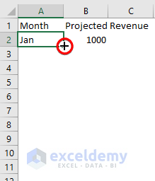
- Click on the Fill Handle icon and drag it downwards (or in the direction you want to copy the cell contents).
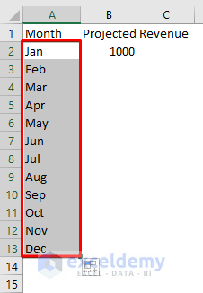
All the month names are Autofilled.
The Fill Handle will Autofill formulas, dates and other series in the same way. A very useful feature indeed.
Method 22 – How to Apply a Formula for Mathematical Operation in Excel
Let’s apply an Excel formula for mathematical calculation. Suppose we want to add a 5% increment to the current month’s value in order to find the next month’s value.
Steps:
- Go to cell B3 and enter the following formula:
B2+B2*5%
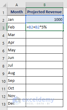
- Press Enter.
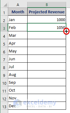
- Drag down the Fill Handle icon.
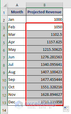
The incremented revenues based on our formula are displayed.
Method 23 – How to Save & Print an Excel Worksheet
How to save a file in Excel?
Steps:
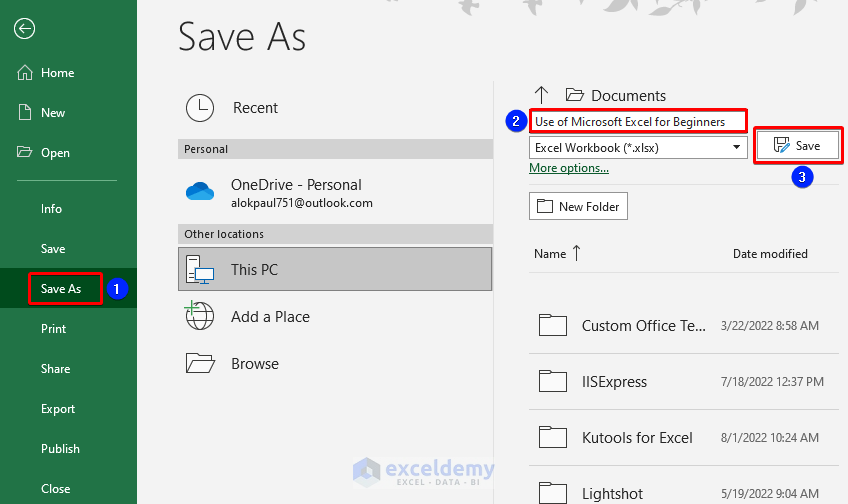
If the file is new or we want to save an existing file afresh, use the Save As feature.
- Click on the File tab.
- Select the Save As option.
- Enter the name of the file in the marked section.
- Click the Save button.
The file name is at the top of the file.
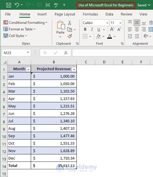
Now, after making modifications to this file, press Ctrl + S to save the file with the same name in the name location.
Now let’s see how to print a saved Excel file.
- Go to File >> Print. Or press Ctrl + P, the keyboard shortcut for opening the Print option.
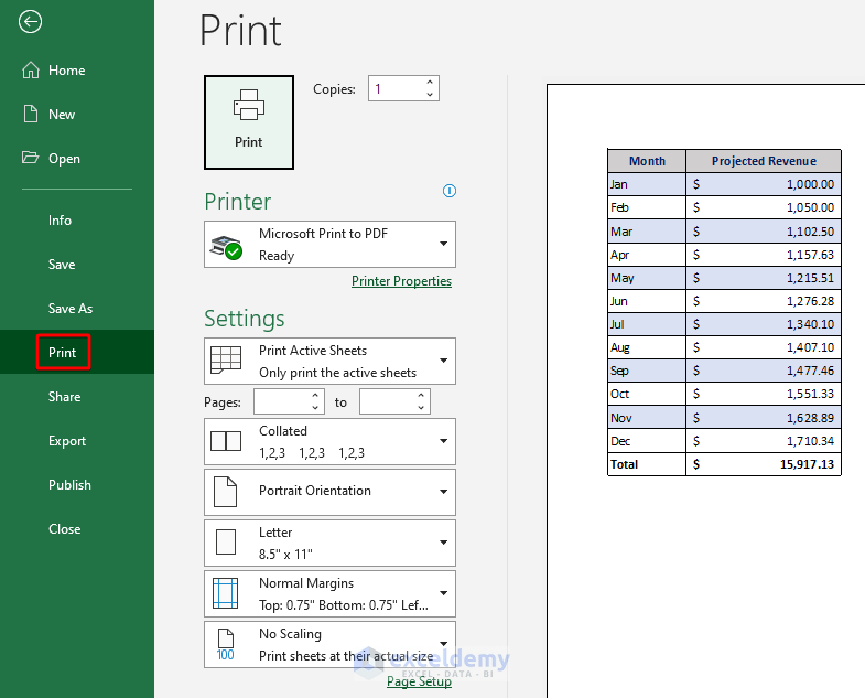
- Choose your options and settings to print as desired.
Method 24 – How to Use Excel’s AutoSave Feature
A devastating situation for beginners (and advanced users!) in Microsoft Excel is when they forget to save their work for a long time, then the file closes or crashes for whatever reason, and their hours of work are lost. Fortunately, Excel provides us with an Autosave feature to save the day.
Steps:
- Go to File >> Options >> Save.
- Set a time for Save AutoRecover information every…minutes.
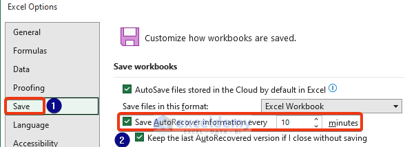
The file will save automatically accordingly.
Method 25 – Some Keyboard Shortcuts to Perform Common Tasks in Microsoft Excel
Finally, for your convenience, here are some of the most commonly used keyboard shortcuts for beginners in Microsoft Excel:
- Ctrl +C – Copy the selection.
- Ctrl +X – Cut the selection.
- Ctrl + V – Paste the selection.
- Ctrl + 1 – Open the Format Cells box.
- F2 – Edit a cell.
- F4 – Toggle the cell reference type between absolute and relative.
- Ctrl + T – Form a table.
Download Practice Workbook
<< Go Back to Learn Excel
Get FREE Advanced Excel Exercises with Solutions!


Great post Kawser.
And thank you for mentioning my Excel Resources page.
It’s my pleasure Rick. Nice to see you here and thanks for commenting!