Implementing Monte Carlo Simulation Using Excel

Monte Carlo Simulation is a statistical technique used to model uncertainty and assess the impact of risk in scenarios like financial forecasting, project management, and inventory analysis. Generating thousands of scenarios Monte Carlo Simulation provides a way to assess variability that helps to make data-driven decisions under uncertainty. In this article, we will implement a Monte Carlo Simulation using Excel.

Let’s define a problem to implement Monte Carlo Simulation. Consider a small e-commerce dataset where you will simulate the profit based on the key metrics that affect the outcomes.

Step 1: Set Up Your Data in Excel

Insert the key metrics in the columns. The key metrics are

• Column A: Simulation Number (1, 2, 3, …, 1000).
• Column B: Selling Price (use RAND function to simulate price per unit).
• Column C: Units Sold (simulate number of units sold).
• Column D: Cost per Unit (random numbers of costing).
• Column E: Calculate Revenue (multiplying units and costs).
• Column F: Total Costs (based on fixed and variable costs).
• Column E: Profit Calculation (subtract revenue and total cost).

Step 2: Generate Random Inputs Using Excel Functions

To generate random numbers for each key variable, you can use RAND, RANDBETWEEN, and NORM.INV functions in Excel.

Simulation No. 

You can use the Series option to insert numbers. Initially insert 1 in Simulation No. column. As we will drag the column it will auto generate the simulation number.

• Select cell A2 and insert 1.

Selling Price:

• Using a normal distribution with a mean of $30 and a standard deviation of $4.5.
• Insert the following formula in cell B2.

Formula:

=NORM.INV(RAND(), 30, 4.5)

This formula generates values that are normally distributed around the mean (30) with a standard deviation of 4.5.

Units Sold:

• Using a Poisson distribution for generating random Poisson values.
• Insert the following formula in cell C2.

Formula:

=RANDBETWEEN(100, 550)

This formula will generate random values within 100 to 550 as units sold of a particular product.

Cost per Unit:

• Generate uniform distribution from $10 to $18.
• Select cell D2 and insert the following formula.

Formula:

=RANDBETWEEN(10, 18)

Revenue:

• To calculate revenue multiply the Units Sold and Selling Price.
• Insert the following formula in cell E2.

Formula:

=B2 * C2

Total Cost:

Calculate total cost as the sum of Fixed Costs, Variable Costs, and Production Costs.

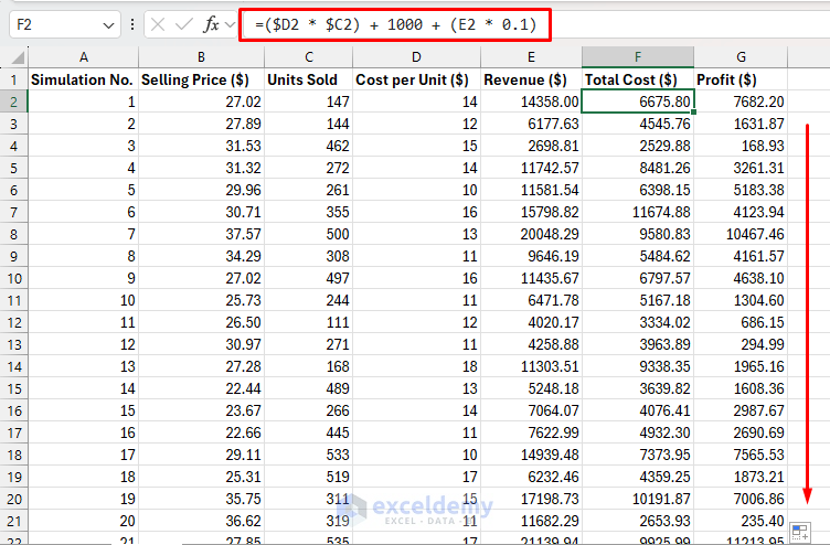
• Select cell F2 and insert the following formula.

Formula:

=($D2 * $C2) + 1000 + (E2 * 0.1)

This formula will calculate the total cost by combining Fixed Costs, Variable Costs, and Production Costs.

• ($D2 * $C2): It’s the variable cost. This part calculates the total cost based on the number of units produced (D2) and the unit cost (C2).
• 1000: is added as a fixed cost, a constant amount regardless of production levels.
• (E2 * 0.1): It calculates the production cost by applying a 10% rate to the Revenue.

Profit:

• To calculate profit, insert the following formula.

Formula:

=E2 - F2

This formula subtracts revenue from total cost.

Output:

You can see all the formulas and results of the variables. Later you can copy all the formulas to generate simulations.

Step 3: Copy Formulas to Create All Simulations

• Drag down the formulas in Columns B, C, D, E, F, and G to generate random data for each simulation.

• Every row will represent one simulation.

Step 4: Analyze the Results

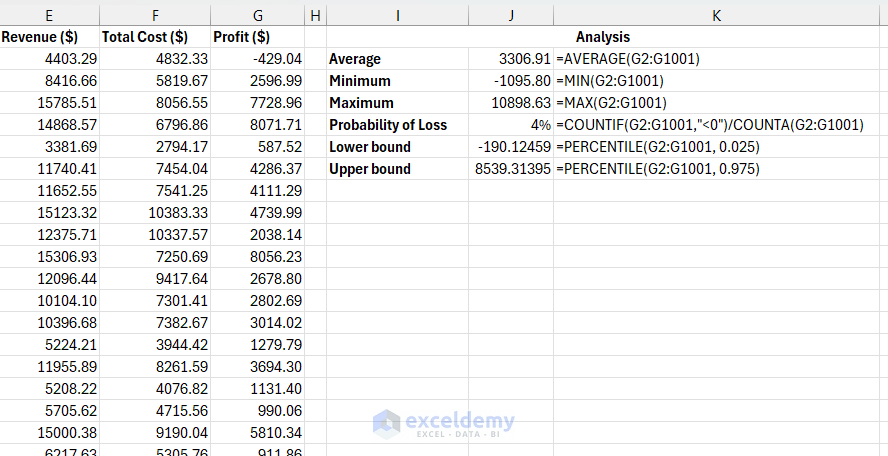
Once the 1000 simulations are generated. let’s analyze the result of the simulations. You can use the following statistical measures to evaluate the profit potential of the business.

Average Profit:

Insert the following formula to calculate the average profit.

Formula:

=AVERAGE(G2:G1001)

The average profit will help you to get the expected result.

Minimum Profit:

Insert the following formula to identify the minimum profit.

Formula:

=MIN(G2:G1001)

The minimum profit will show you the worst-case scenario.

Maximum Profit:

Use the following formula to identify the maximum profit.

Formula:

=MAX(G2:G1001)

The maximum profit will show you the best possible outcome.

Probability of Loss:

Calculate the percentage of simulations where the profit is negative.

Formula:

=COUNTIF(G2:G1001,"<0")/COUNTA(G2:G1001)

It will help you to get an idea of how much loss you may face.

95% Confidence Interval (CI) for Profit:

Calculate the lower and upper bounds of the 95% CI.

Lower bound:

=PERCENTILE(G2:G1001, 0.025)

This formula calculates the 2.5th percentile which means 2.5% of the profit data falls below this value.

Upper bound:

=PERCENTILE(G2:G1001, 0.975)

This formula calculates the 97.5th percentile which means 97.5% of the profit data falls below this value.

Output:

Create a Histogram of Profit:

• Select the Profit column.
• Go to the Insert tab >> from Charts >> select Histogram.

You will get the Histogram for Profit column.

The distribution of profits shows how profits are spread.

Monte Carlo Simulation Using the Data Table Tool

You can use the Data Table tool to implement Monte Carlo Simulation. You can use the Series option to insert simulation numbers.

• Create a Data Table with the column name.
• Insert 1 in cell A2 of Simulation No. column.
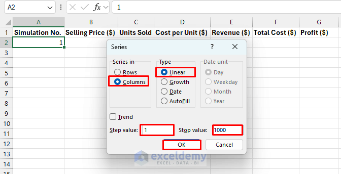
• Go to the Home tab >> from Fill >> select Series.

• In the Series dialog box;
  • Series in: Columns
  • Type: Linear
  • Step value: 1
  • Stop Value: 1000
  • Click OK.

• Select the entire table from the A2:G1001 cell.
• Go to the Data tab >> from What-If_Analysis >> select Data Table.

• In the Data Table dialog box;
  • Row input cell: Keep it blank.
  • Column input cell: Select A2 cell.
  • Click OK.

The Data Table will generate 1000 simulation values.

Tips and Best Practices

• Use cell references for variable limits to update easily.
• Set your Calculation Mode to Manual. Otherwise, data will update every time you hit Enter. To calculate the cells use Calculate Now (F9) option.
• Run at least 1000 to 10,000 simulations for more accurate predictions.
• If you need to run tens of thousands of simulations, VBA can handle them more efficiently.

Conclusion

By following all the steps you can implement Monte Carlo Simulation in Excel. It is a versatile method to predict possible outcomes under uncertainty. By using Excel’s RANDBETWEEN, RAND, and NORM.INV functions, you can build robust models to analyze risks and improve decision-making. Monte Carlo Simulation helps to analyze financial risk, optimize project timelines, etc.