How to Import Data from Excel to Google Sheets Using the IMPORTRANGE Function

Overview of the IMPORTRANGE Function

Function Objective

The IMPORTRANGE function allows you to retrieve specific ranges of values from an Excel worksheet and import them into a Google Sheet. It’s important to note that this function is only available in Google Sheets.

Syntax

=IMPORTRANGE([spreadsheet_url], [range_string])

Arguments Explanation

Argument	Required/Optional	Explanation
spreadsheet_url	Optional	This is the web link or URL of the source workbook from which you want to import data into a new worksheet.
range_string	Optional	Specify the specific cell or range of cells that you want to import from the original data.

Since the IMPORTRANGE function is not available in Excel, we need to first import the Excel workbook into Google Sheets. Without this step, we won’t be able to transfer data using the function. Let’s dive into the methods for using the IMPORTRANGE function.

Method 1 – Applying IMPORTRANGE Function in Google Sheets for Importing a Single Worksheet from Excel

In this method, we’ll use the IMPORTRANGE function for a single worksheet. There are two ways to do this:

1.1. Use of URLs or Spreadsheet Keys

Import the Excel file into Google Sheets:
- Open a blank sheet in Google Sheets.
- Go to the File tab and select Import.

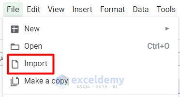
- Choose your required file from Google Drive.
- Select the type of import location from the drop-down menu and click Import data.

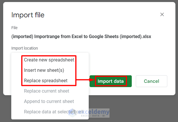
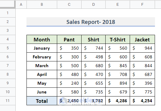
- The Excel workbook is now in Google Sheets.

Copy the shortcode from the URL of the source dataset (press Ctrl + C on your keyboard).

Enter the IMPORTRANGE function in Cell B4 of a new sheet and paste the URL within two quotation marks, like this:

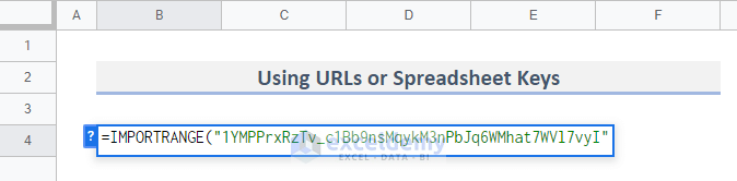
Along with the URL, insert the sheet name and cell range (B4:F11) according to the source dataset.

=IMPORTRANGE("1YMPPrxRzTv_c1Bb9nsMqykM3nPbJq6WMhat7WVl7vyI","2018!B4:F11")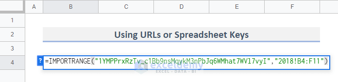

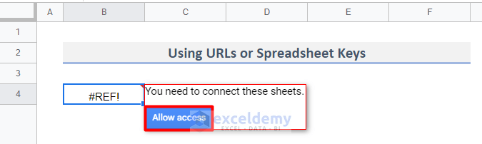
You’ll encounter a #REF! error, which prompts you to give access for connecting both sheets. Press Allow access.

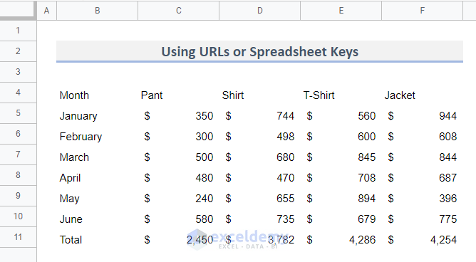
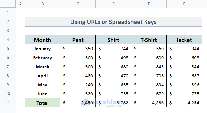
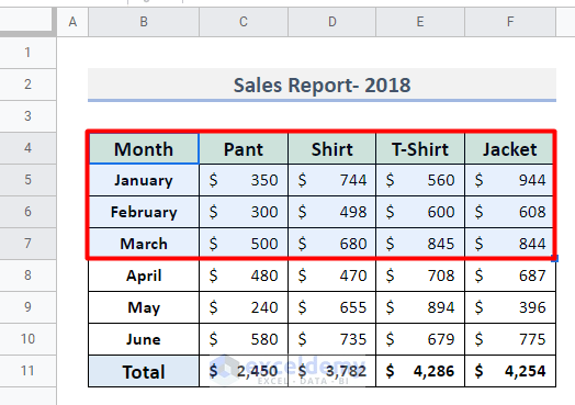
Finally, you’ll get the data imported all at once. After formatting, the data table will look like this:

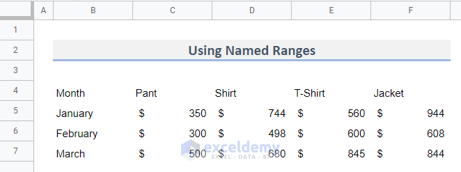
After some formatting, the data table looks like this.

Note: When you press “Allow access” in a worksheet, it applies to the entire file. Regardless of how many worksheets you add later, it will fetch data from the URL without further permission requests.

1.2. With Named Ranges

Select the cell range B4:F7 in the source dataset.

Right-click on it and go to View more cell actions.
From the Context Menu, select the option Define named range.

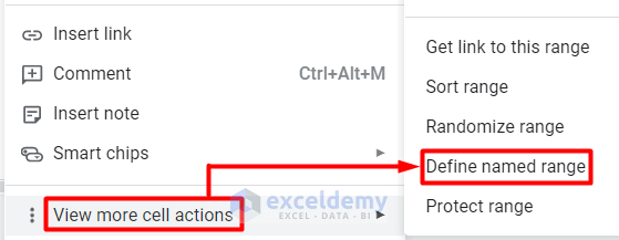
Provide a name for that specific range and click Done.

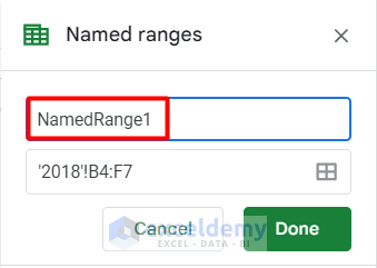
Now, enter this formula in Cell B4 of the new sheet.

=IMPORTRANGE("1YMPPrxRzTv_c1Bb9nsMqykM3nPbJq6WMhat7WVl7vyI","NamedRange1")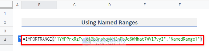

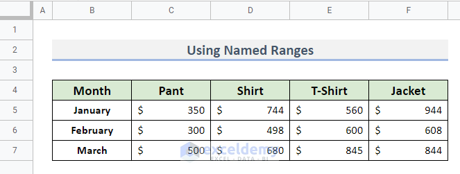
Press Enter, and you’ll get the output.

Format the dataset to achieve the final result.

Method 2 – Using the IMPORTRANGE Function to Extract Data from Multiple Worksheets in Excel to Google Sheets

We can apply the IMPORTRANGE function to transfer data from multiple Google worksheets. Let’s explore how it works:

2.1. Using Arrays

When transferring data from multiple sheets simultaneously, we create an array formula that works as a group. Follow these steps:

Insert the following formula in Cell B4 of the new sheet:

={IMPORTRANGE("1YMPPrxRzTv_c1Bb9nsMqykM3nPbJq6WMhat7WVl7vyI","2018!B4:F10");IMPORTRANGE("1YMPPrxRzTv_c1Bb9nsMqykM3nPbJq6WMhat7WVl7vyI","2019!B5:F10")}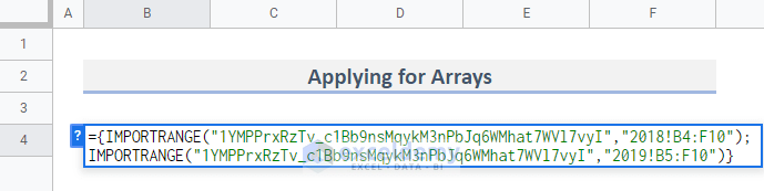

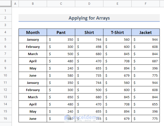
Note: You can add more sheet references to this formula. Ensure that you insert the correct sheet names and cell ranges in each argument.

Press Enter.

You will now have the dataset from two worksheets combined into a single one.

2.2. Using the QUERY Function

We can also combine the QUERY function with IMPORTRANGE to retrieve data from multiple sheets. The QUERY function allows you to filter data based on specific conditions and reorder columns. Follow these steps:

Enter the following formula in Cell B4:

=QUERY({IMPORTRANGE("1YMPPrxRzTv_c1Bb9nsMqykM3nPbJq6WMhat7WVl7vyI","2018!B4:F10");IMPORTRANGE("1YMPPrxRzTv_c1Bb9nsMqykM3nPbJq6WMhat7WVl7vyI","2019!B5:F10")},"select * where Col1 is not null")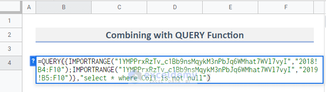

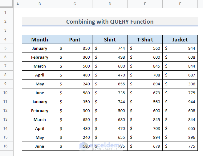
Press Enter.
You will obtain the final output.

In this formula, the IMPORTRANGE function imports data from other Google sheets using the provided URLs and cell ranges. The QUERY function then filters the data based on the condition where column 1 is not null.

Errors while Using IMPORTRANGE Function

You may encounter various errors while using IMPORTRANGE. Here are two common ones and their reasons:

Error #N/A: Occurs when the formula has incorrect arguments or when URLs/cell ranges are not enclosed in quotes.
Error: #REF!: Appears when the URL requires access permission. Even if the Google Sheet is not in Editor mode, this error will occur.

Things to Remember

Enclose each argument in quotes to avoid errors.
Changes made in the original worksheet will automatically update in the new sheet where the IMPORTRANGE function is applied.
Data synchronization occurs in one direction; attempting to modify data in the new sheet will result in an error.
You can use entire column references instead of cell ranges in the formula.

<< Go Back to Export Excel to Google Sheets | Export Data from Excel | Learn Excel

Get FREE Advanced Excel Exercises with Solutions!