Method 1 – Use of INDEX MATCH Functions across Multiple Sheets in Excel
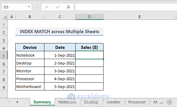
In the following picture, you can see multiple worksheets open in a single workbook. The first sheet has been named as Summary. In this sheet, the sales of a particular device or component on a particular date will be extracted from other corresponding worksheets.
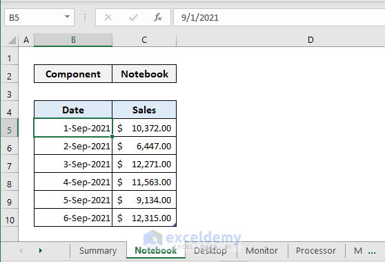
Below is the screenshot of the second worksheet named Notebook where the sales of notebooks on some successive dates have been recorded. Similarly, if we go through the rest of the worksheets available then we’ll find the sales of other devices or components- Desktop, Monitor, Processor, and Motherboard.
In the Summary sheet, we’ll extract the sales of notebooks on 1-Sep-2021 from the Notebook sheet.
Step 1:
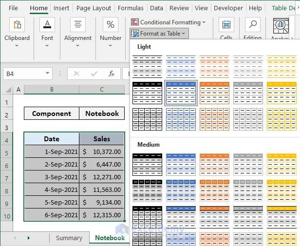
➤ In the Notebook worksheet, select the entire table.
➤ From the Styles group of commands under the Home ribbon, select any table you prefer from the Format as Table drop-down.
Step 2:
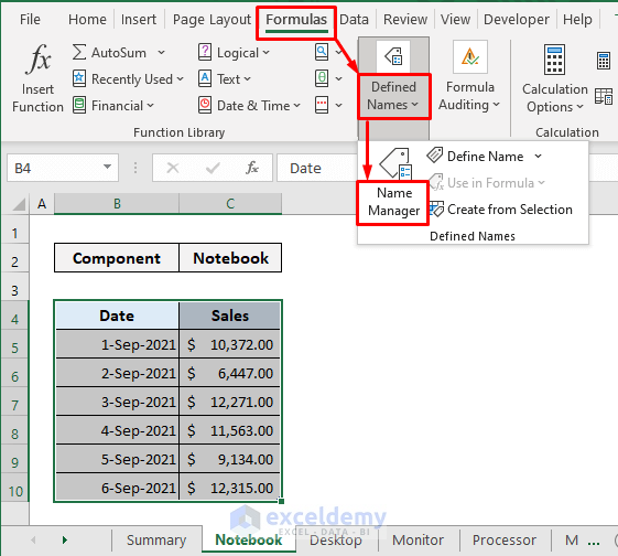
➤ Go to the Formulas tab and select the Name Manager command from the Defined Names drop-down.
Step 3:
➤ Edit the name of the table here and type Notebook in the Name box.
➤ Press OK.
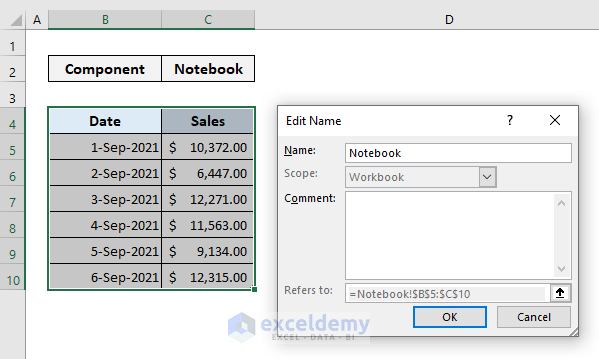
Step 4:
➤ Follow the previous step for all other worksheets and name the corresponding tables with the device or components present in the Summary sheet.
➤ Close the Name Manager dialogue box and you’re now ready to assign the formula in the Summary sheet.
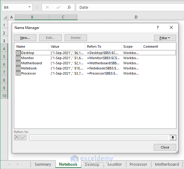
Step 5:
➤ In the first output Cell D5, type the following formula:
=INDEX(INDIRECT(B5&"[Sales]"),MATCH(Summary!$C5,INDIRECT(B5&"[Date]"),0))➤ Press Enter and you’ll get the sales value of notebooks on 1-Sep-2021.
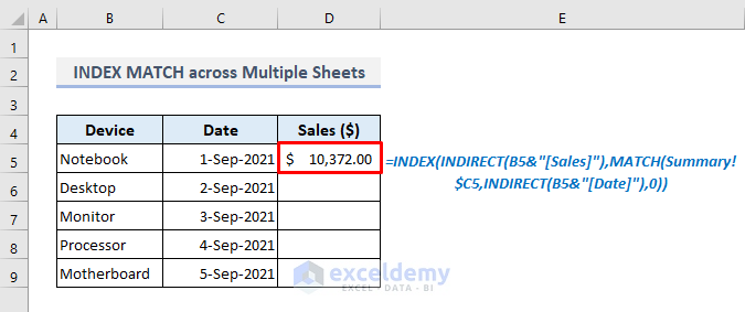
Step 6:
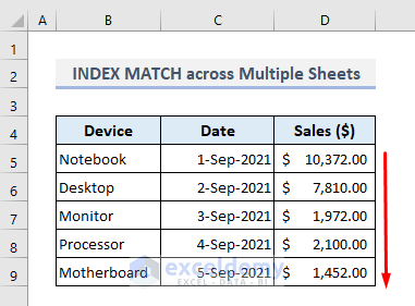
➤ Use Fill Handle to fill down the rest of the cells in Column D.
You’ll see the display the sales of other components or devices on the specified dates. If you change a date for any device in Column C, you’ll find the sales value of the particular device on that specified date at once. Similarly, you can change the device name too in Column B and you’ll be shown the corresponding sales value on the particular date.
Method 2 – Use (VLOOKUP) Instead of the INDEX MATCH Functions across Multiple Sheets
There is a suitable alternative to the INDEX and MATCH functions and that is the VLOOKUP function. The VLOOKUP function looks for a value in the leftmost column of a table and then returns a value in the same row from a specified column.
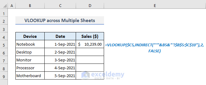
Since we’re using the previous dataset, let’s have a look at how we can apply the VLOOKUP function in the output Cell D5 now. The required formula is:
=VLOOKUP($C5,INDIRECT("'"&B5&"'!$B$5:$C$10"),2,FALSE)After pressing Enter only, you’ll get the first output as found in the previous method.
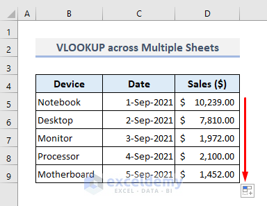
Use the Fill Handle option to autofill the rest of the output cells in Column D and you’ll be displayed the corresponding sales values right away.
Download Practice Workbook
You can download the Excel workbook that we’ve used to prepare this article.
<< Go Back to INDEX MATCH | Formula List | Learn Excel
Get FREE Advanced Excel Exercises with Solutions!

