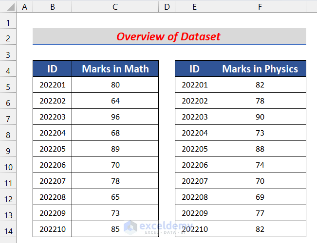
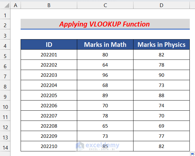
Consider two tables with examination marks in math and physics.
Method 1 – Applying the VLOOKUP Function to perform an Inner Join in Excel
Steps:
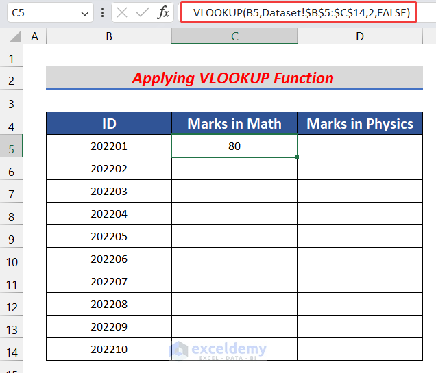
- In a new sheet, store all IDs in B5:B14.
- Select C5 and enter the following formula:
=VLOOKUP(B5,Dataset!$B$5:$C$14,2,FALSE)
- Press Enter.
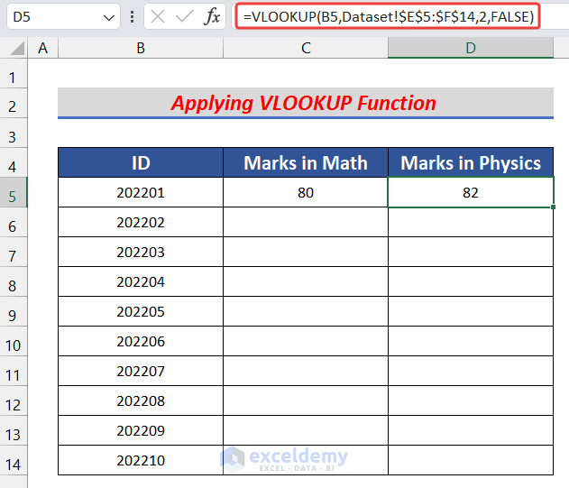
- Select D5 and use the following formula:
=VLOOKUP(B5,Dataset!$E$5:$F$14,2,FALSE)
- Press Enter.
- Select C5:D5 and drag down the Fill Handle to copy the formula to the rest of the cells.
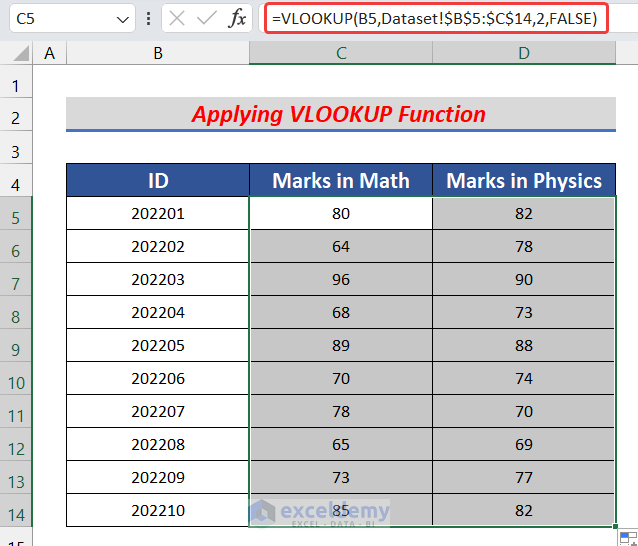
This is the output.
Method 2 – Using the Power Query Feature to perform an Inner Join in Excel
Steps:
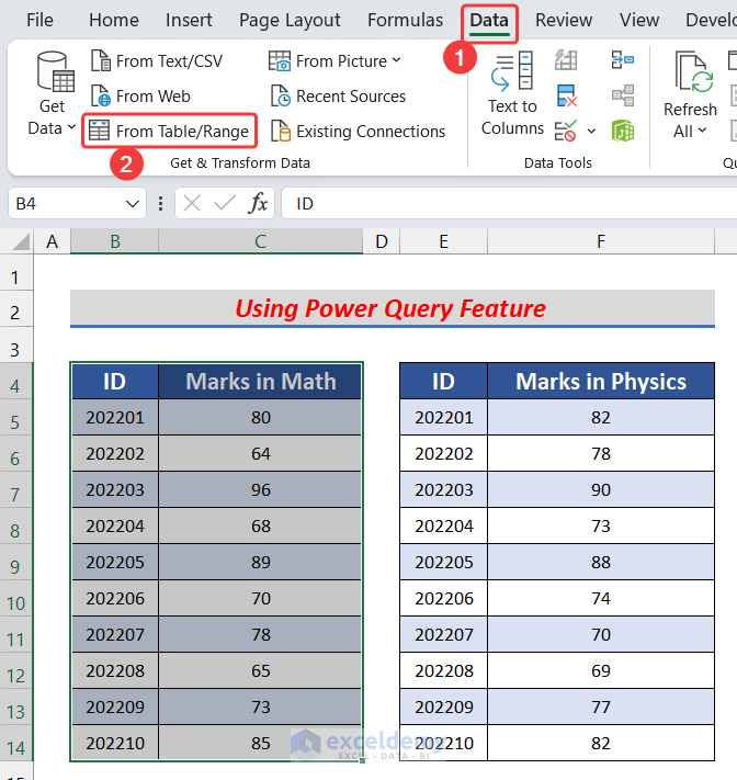
- Select B4:C14.
- In the Data tab, click From Table/Range in Get & Transform.
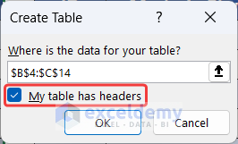
- In the Create Table dialog box, check My table has headers.
- Click OK.
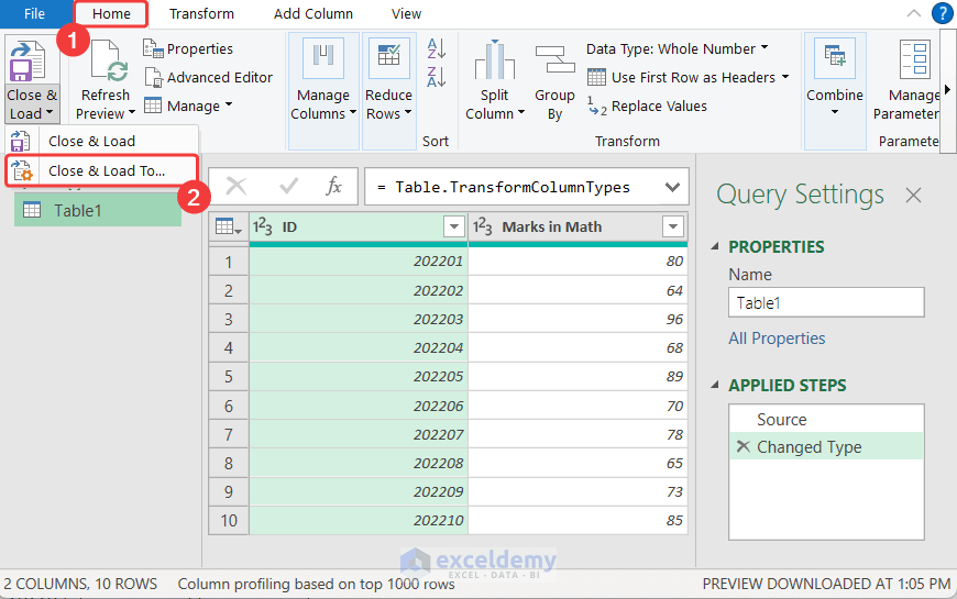
- The Power Query Editor will be displayed.
- In the Home tab, click Close & Load and choose Close & Load To.
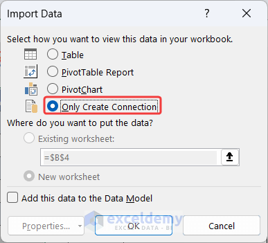
- In Import Data, choose Only Create Connection.
- Click OK.
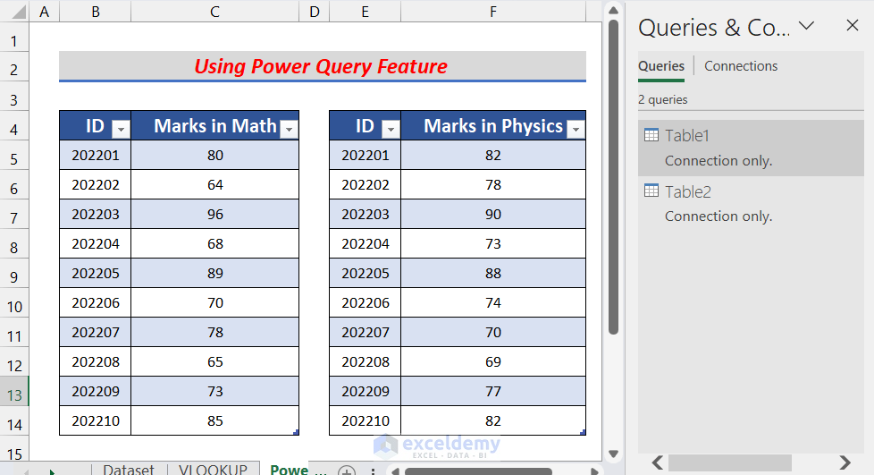
- Follow the same procedure for the second table to create a connection.
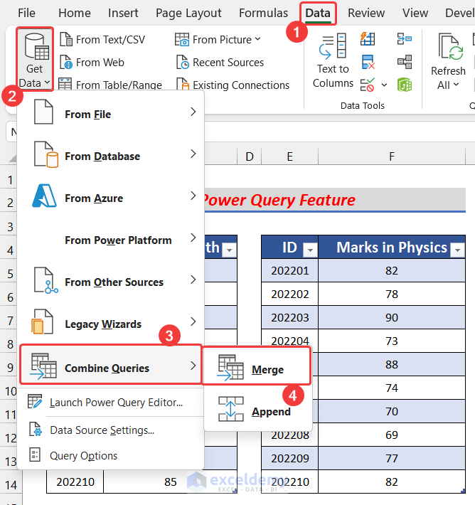
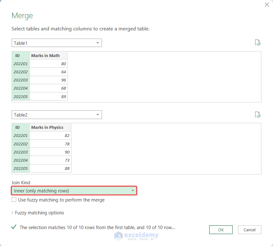
- In the Data tab, click Get Data and choose Combine Queries > Merge.
- In the Merge dialog box, click the drop-down arrow and select Table1.
- Click the ID column.
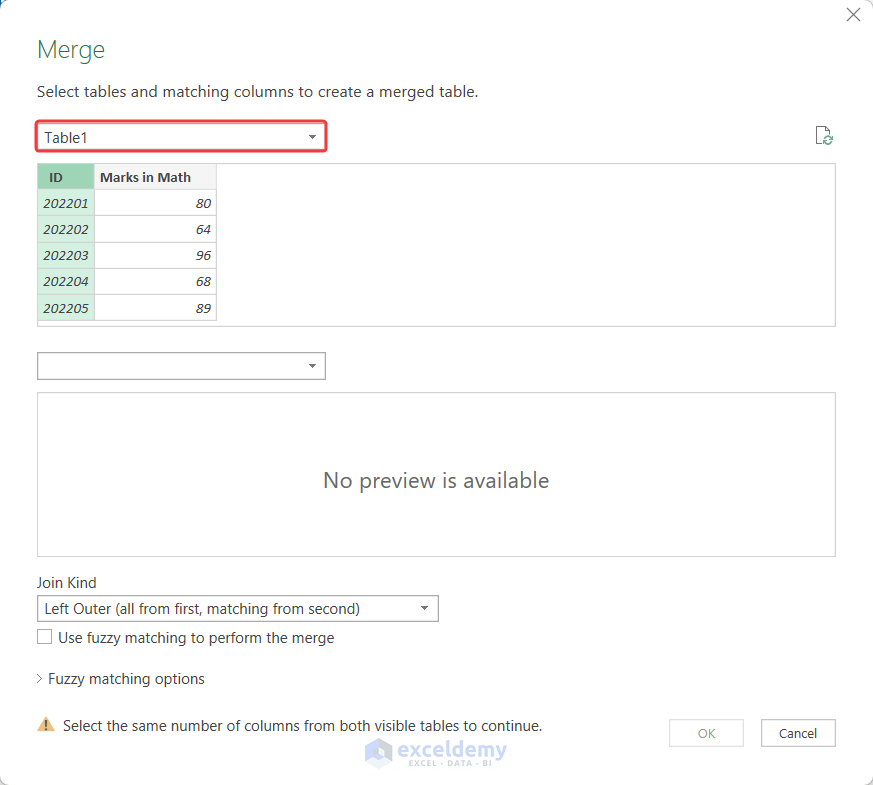
- Follow the same procedure in the lower field.
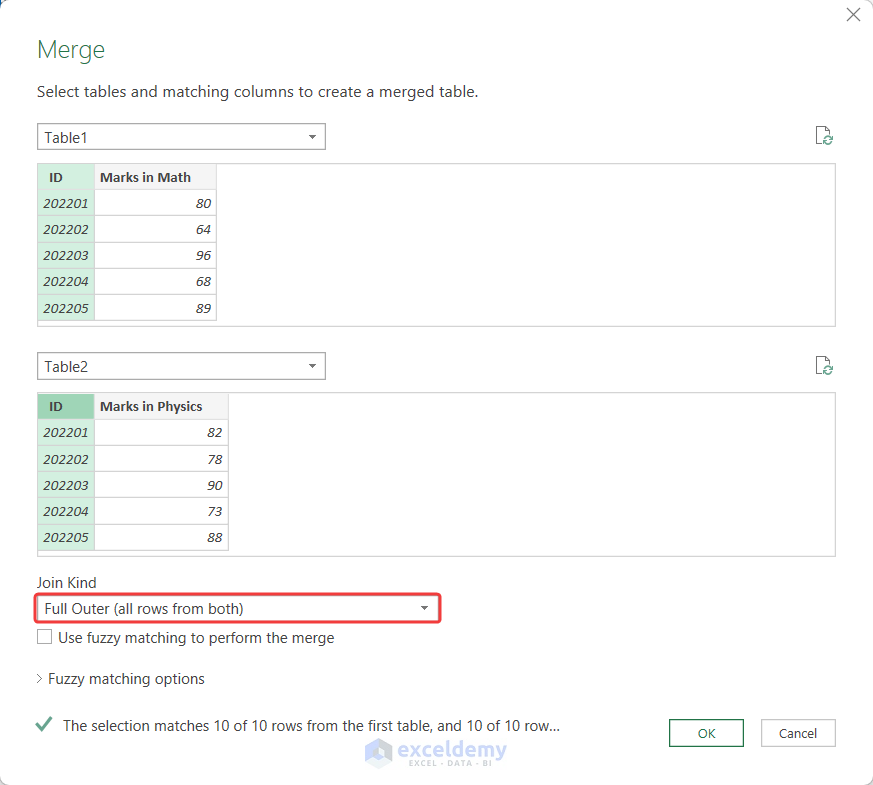
- In Join Kind, select Inner (only matching rows).
- Click OK.
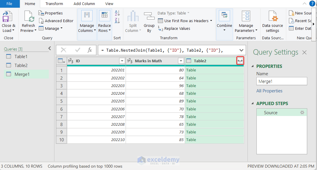
- In the Power Query Editor table, click the expand icon in the heading of Table2.
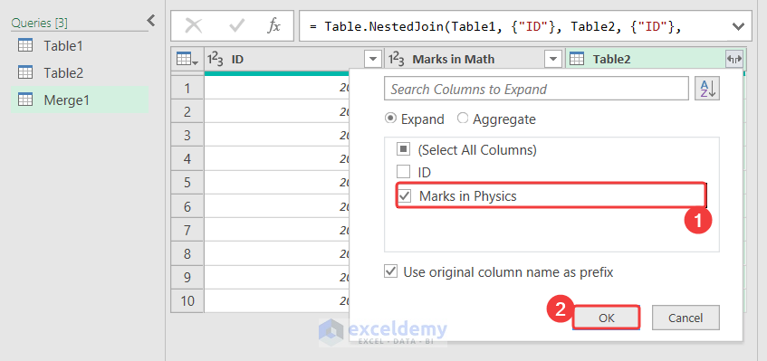
- Uncheck ID and click OK.
- In the Home tab, click Close & Load.
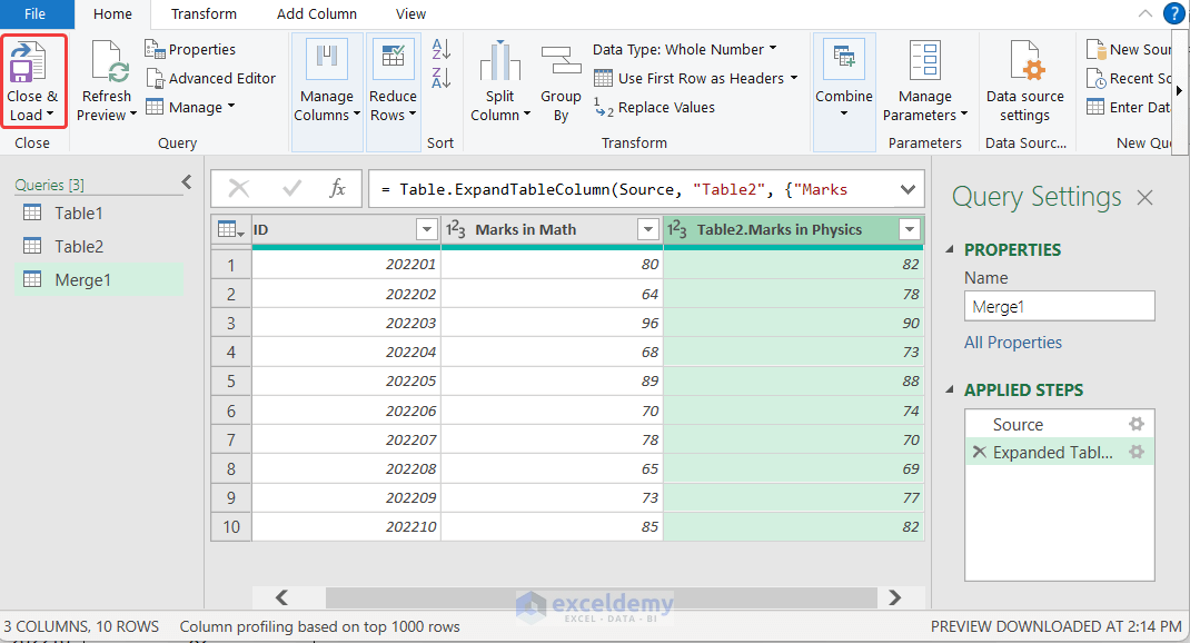
A new sheet will open, showing the joined table.
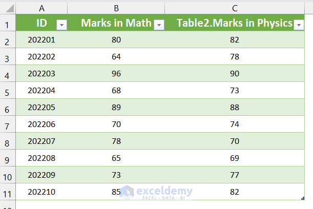
To outer join in Excel, choose Full Outer (all rows from both) in Join Kind.
Read More: How to Combine Two Tables Using Power Query in Excel
How to perform Left Join in Excel
The dataset is in B5:G14.
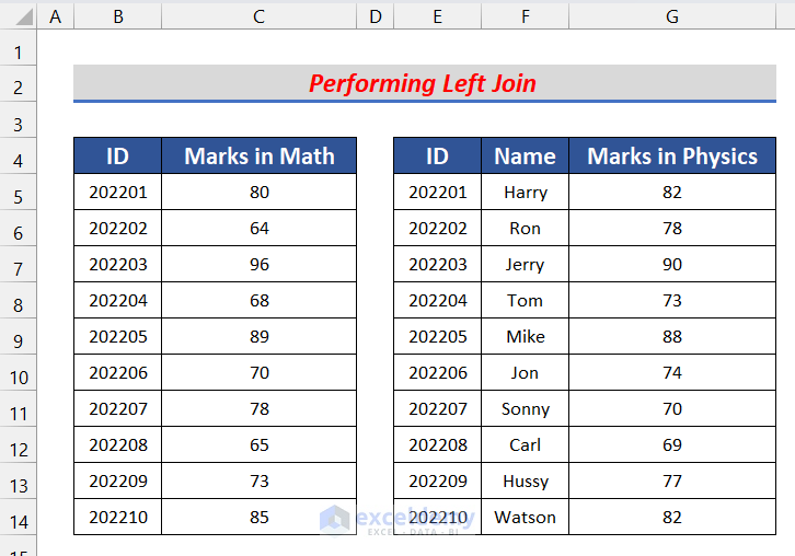
Steps:
- In a new sheet, store the first table in B5:C14.
- Select D5 and use the following formula:
=VLOOKUP('Left Join'!B5,Left!$E$5:$G$14,{2,3},FALSE)
- Press Enter.
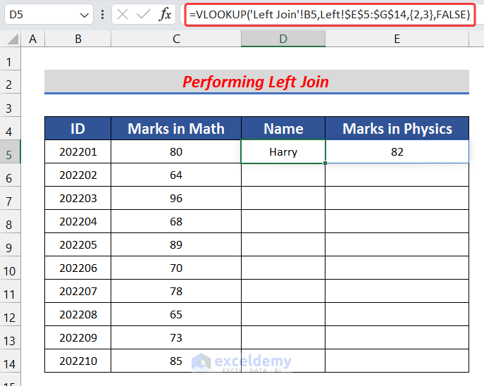
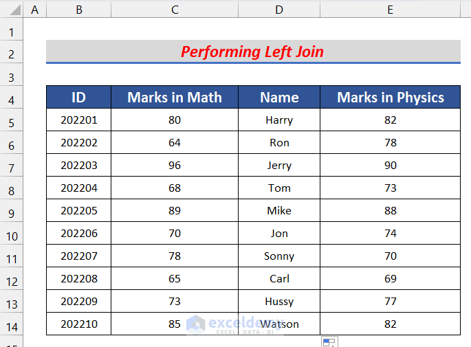
- Drag down the Fill Handle to see the result in the rest of the cells.
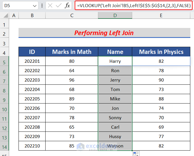
This is the output.
Download Practice Workbook
Download the practice workbook.
Related Articles
- How to Perform Left Outer Join in Excel
- How to Create Full Outer Join in Excel
- How to Create Cross Join in Excel
<< Go Back to Power Query Excel | Learn Excel
Get FREE Advanced Excel Exercises with Solutions!

