In the following dataset, we will count the Total Sales from 2015 to 2020 for different months. However, we have missed including the Sales for 2016. So, we need to insert a column between the data sets. To do so, we will take two approaches: applying the INDIRECT function and the INDEX function.
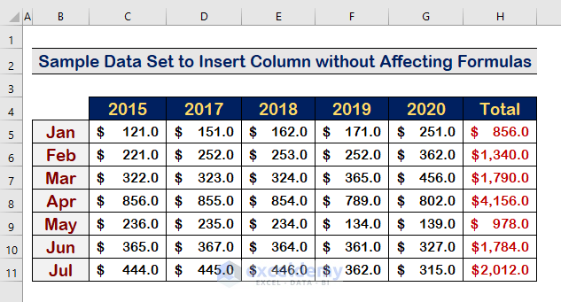
Method 1 – Apply the INDIRECT Function to Insert Column without Affecting Formulas
Step 1: Use the INDIRECT Function
- Insert the following formula of the INDIRECT function with the SUM function to sum the range C5 to G5:
=SUM(INDIRECT("C5:G5"))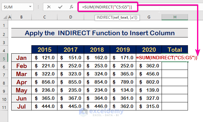
Step 2: Apply the INDIRECT Function in Each Cell in a Column
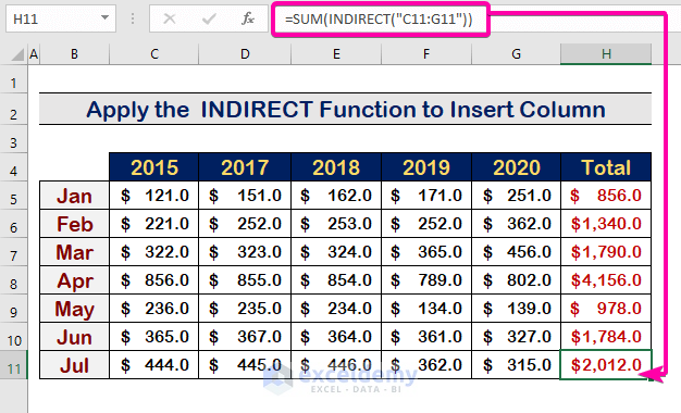
- Apply the same function according to the cell references for each cell.
- The Total column will appear, as shown in the image below.
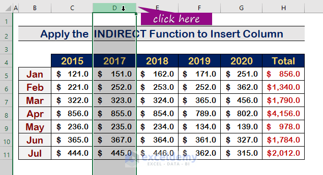
Step 3: Select a Column
- Click on the D to select the entire column.
Step 4: Insert a Column
- Right-click the mouse.
- Click on Insert.
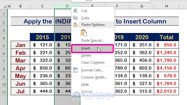
- As a result, you can insert a new column to the left, and your newly added column will show as in the image below.
- The formula in cell I5 remains unchanged.
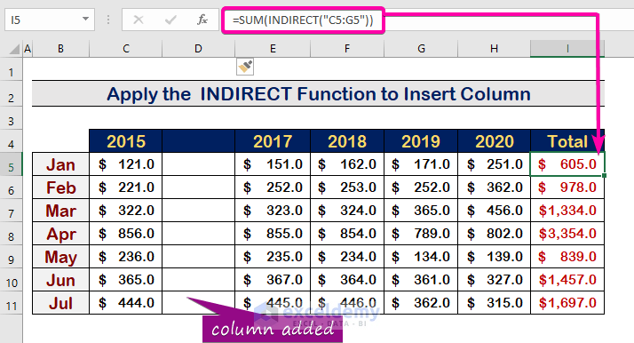
Step 5: Final Result
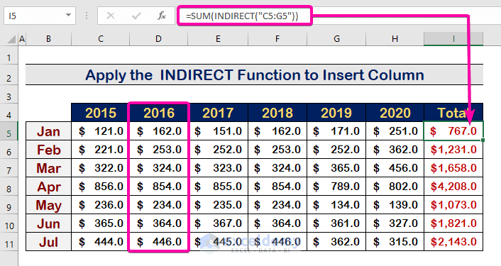
- Add the value for the year 2016 in the new column.
- It will keep the formula in cell I5 and change the value according to the formula.
Read More: Insert a Column Between Every Other Column in Excel
Method 2 – Use the INDEX Function to Insert Columns without Affecting Formulas
Step 1: Insert the Array Argument of the INDEX Function
- To apply the INDEX function in the worksheet, use cells 1 to 65526 as an array with the following formula.
=SUM(INDEX($1:$65536,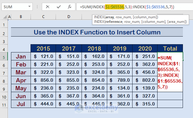
Step 2: Enter the row_num Argument of the INDEX Function
- Insert the row no. of the first reference cell C5 as 5.
=SUM(INDEX($1:$65536, 5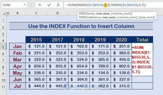
Step 3: Type the column_num Argument of the INDEX Function
- Enter column_num as 3 for the reference cell C5.
=SUM(INDEX($1:$65536,5,3)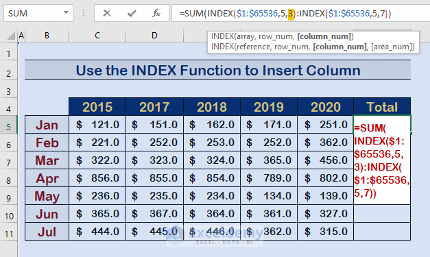
Step 4: Enter the Array Argument of the INDEX Function
- Enter $1:$65536 to select the entire sheet.
=SUM(INDEX($1:$65536,5,3):INDEX($1:$65536,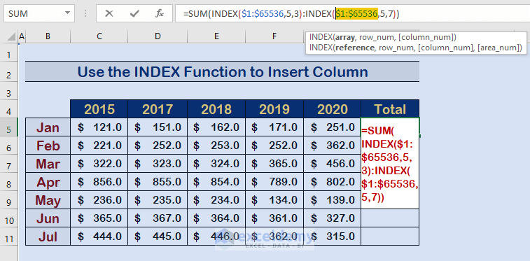
Step 5: Write the row_num Argument of the INDEX Function
- Type 5 as the row number for cell G5, and as the second reference cell, row_num is 5.
=SUM(INDEX($1:$65536,5,3):INDEX($1:$65536,5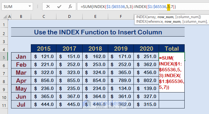
Step 6: Write the column_num Argument of the INDEX Function
- Insert 7 as the column number of the second cell reference.
=SUM(INDEX($1:$65536,5,3):INDEX($1:$65536,5,7)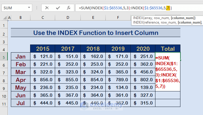
Step 7: Final Formula to Sum
- The formula becomes:
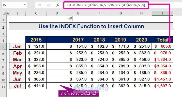
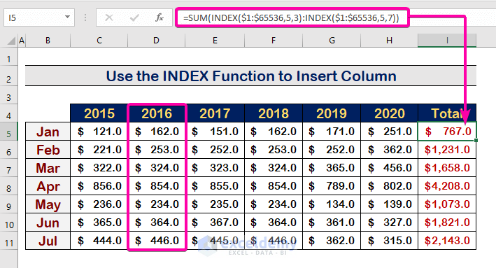
=SUM(INDEX($1:$65536,5,3):INDEX($1:$65536,5,7))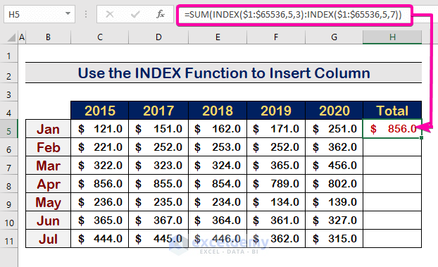
Step 8: Apply Formulas for Each Cell in the Column
- Repeat the pattern for the other cell references with the following formula:
(For example – cells C11 to G11)
=SUM(INDEX($1:$65536,11,3):INDEX($1:$65536,11,7))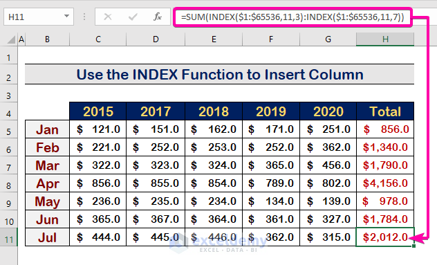
Step 9: Select a Column
- Click on the D to select the whole column.
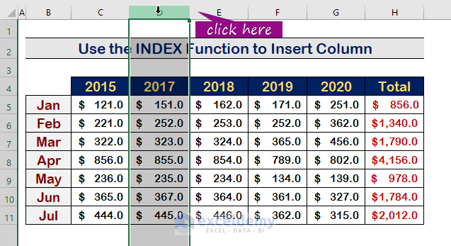
Step 10: Insert a Column
- Right-click the mouse and click on the Insert.
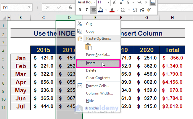
- Your new column has been added, and the formula remains the same.
- Type anything between the columns that will adjust the value while keeping the formula.
Read More: Excel Fix: Insert Column Option Greyed out
Download the Practice Workbook
Download this practice workbook to exercise while you are reading this article.
Related Articles
<< Go Back to Columns in Excel | Learn Excel
Get FREE Advanced Excel Exercises with Solutions!

